| PREVIOUS | INDEX | NEXT |
| Optics | Wolter Type-I | |||||||||
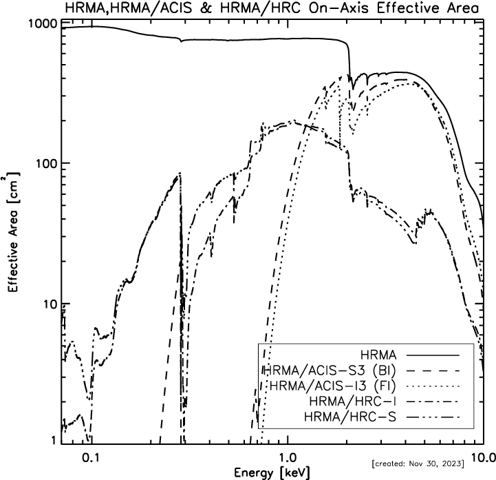
| Mirror coating | Iridium (330 Å, nominal) | |||||||||
| Mirror outer diameters (1, 3, 4, 6) | 1.23, 0.99, 0.87, 0.65 m | |||||||||
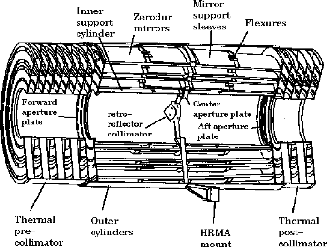
| Mirror lengths (Pn or Hn) | 84 cm | |||||||||
| Total length (pre- to post-collimator) | 276 cm | |||||||||
| Unobscured clear aperture | 1145 cm2 | |||||||||
| Mass | 1484 kg | |||||||||
| Focal length | 10.070 ±0.003 m | |||||||||
| Plate scale | 48.82 ±0.02 μm arcsec−1 | |||||||||
| Exit cone angles from each hyperboloid: | ||||||||||
| θc (1, 3, 4, 6) | 3.42°, 2.75°, 2.42°, 1.80° | |||||||||
| θd (1, 3, 4, 6) | 3.50°, 2.82°, 2.49°, 1.90° | |||||||||
| f-ratios (1, 3, 4, 6) | 8.4, 10.4, 11.8, 15.7 | |||||||||
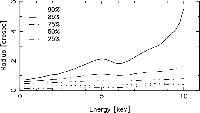
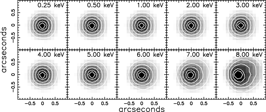
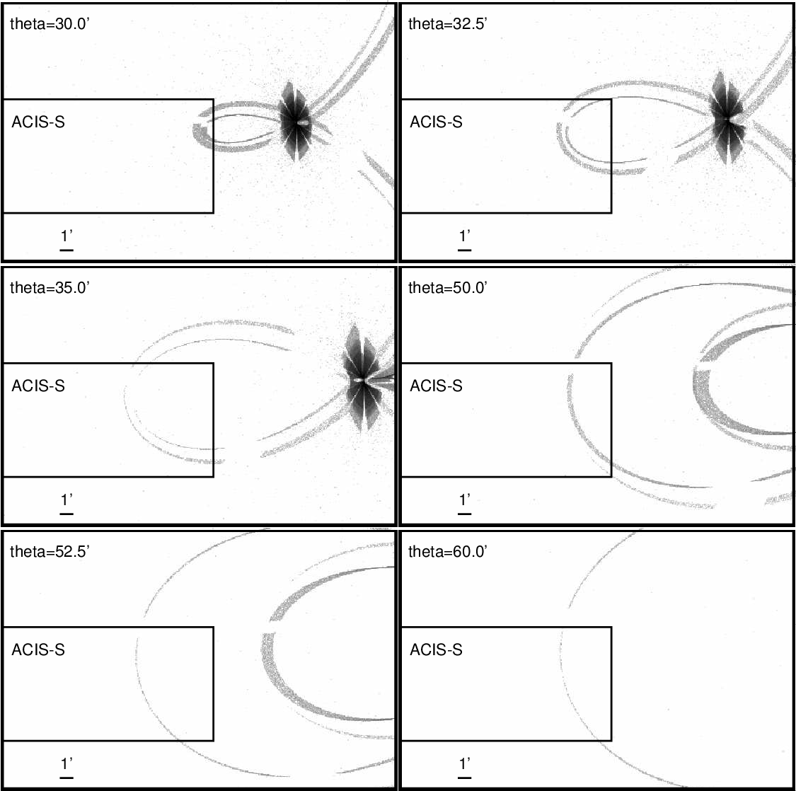
| PSF FWHM (with detector) | < 0.5 arcsec | |||||||||
|
| |||||||||
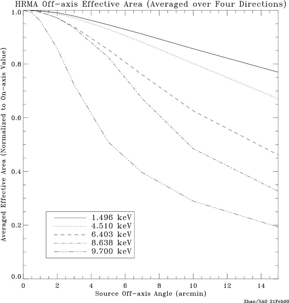
| Ghost-free field of view | 30 arcmin diameter |
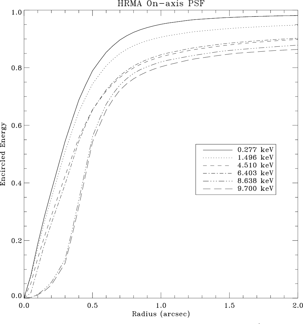
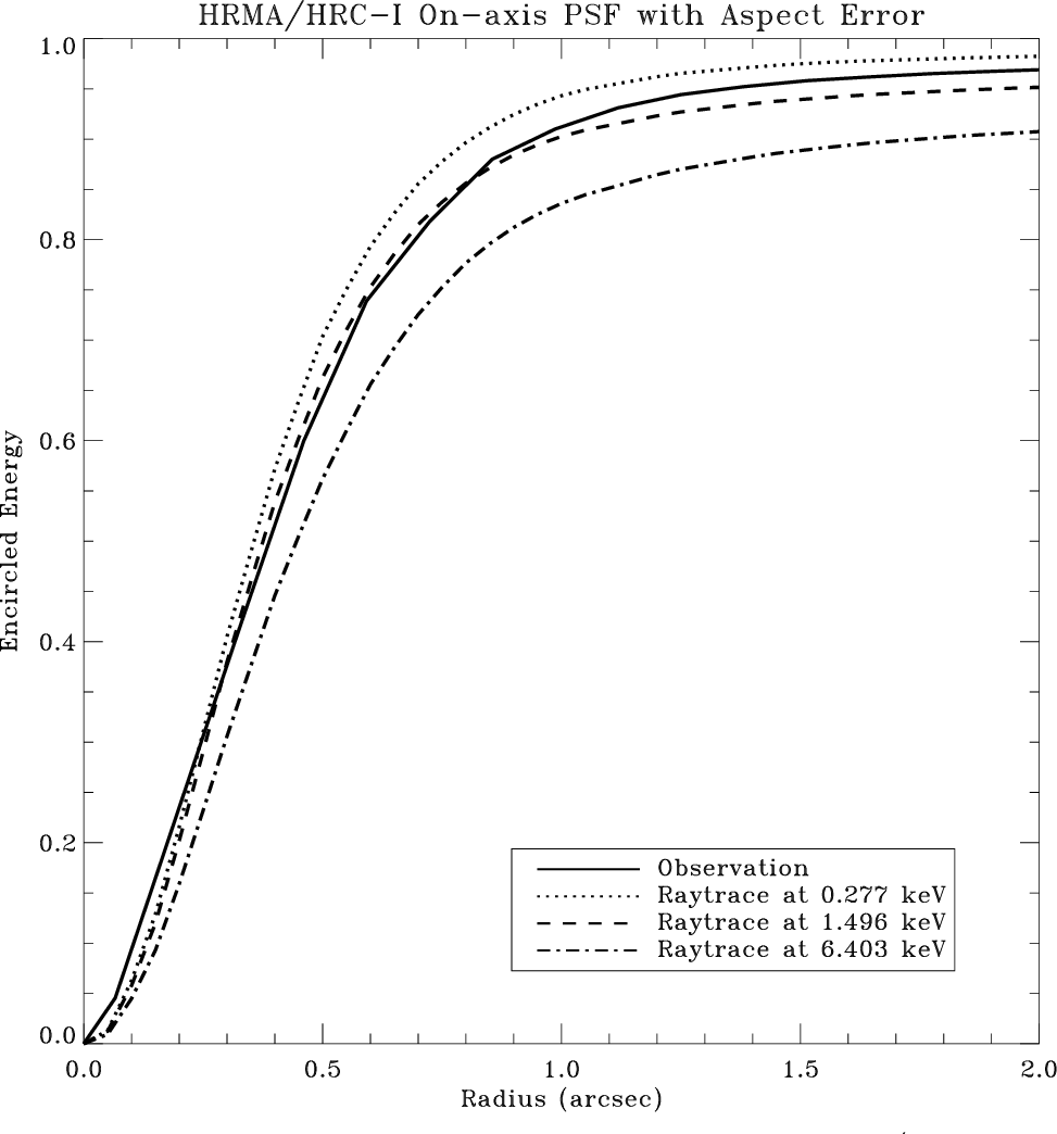
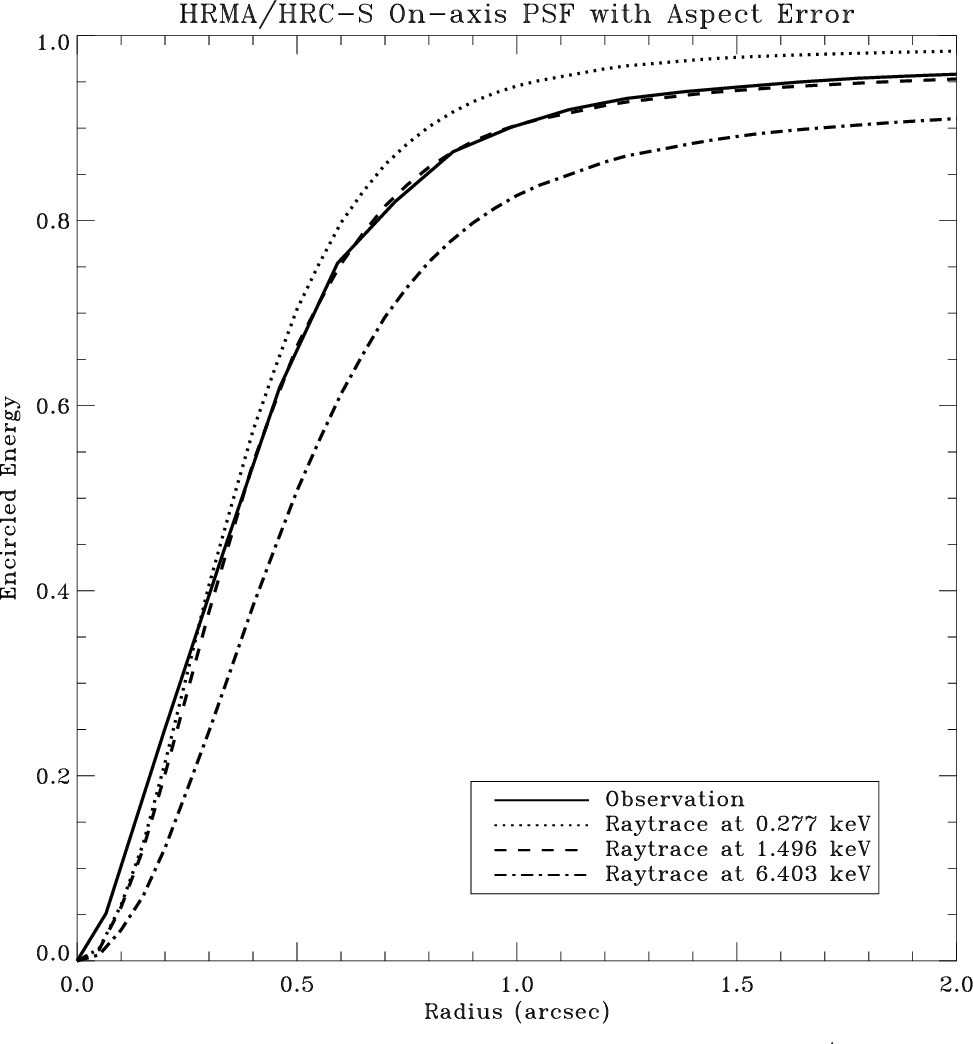
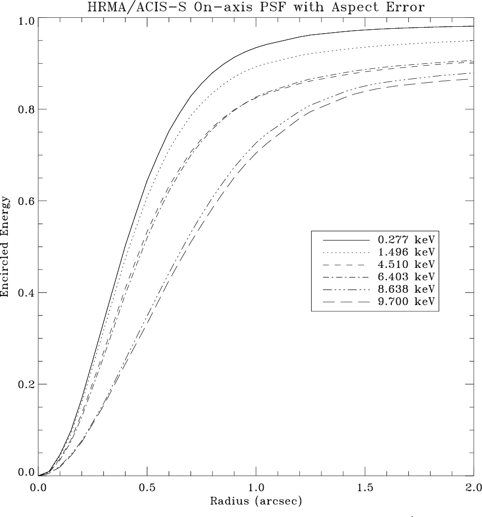
| X-ray: | Encircled Energy Fraction | ||
| E | λ | Diameter | |
| keV | Å | 1 arcsec | 10 arcsec |
| 0.1085 | 114.2712 | 0.7954 | 0.9979 |
| 0.1833 | 67.6401 | 0.7937 | 0.9955 |
| 0.2770 | 44.7597 | 0.7906 | 0.9929 |
| 0.5230 | 23.7064 | 0.7817 | 0.9871 |
| 0.9297 | 13.3359 | 0.7650 | 0.9780 |
| 1.4967 | 8.2838 | 0.7436 | 0.9739 |
| 2.0424 | 6.0706 | 0.7261 | 0.9674 |
| 2.9843 | 4.1545 | 0.6960 | 0.9560 |
| 3.4440 | 3.6000 | 0.6808 | 0.9479 |
| 4.5108 | 2.7486 | 0.6510 | 0.9319 |
| 5.4147 | 2.2898 | 0.6426 | 0.9300 |
| 6.4038 | 1.9361 | 0.6365 | 0.9344 |
| 8.0478 | 1.5406 | 0.5457 | 0.9185 |
| 8.6389 | 1.4352 | 0.5256 | 0.9151 |
| 10.0000 | 1.2398 | 0.4971 | 0.8954 |
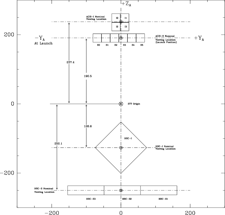
| Detector | Chip | SIM-Z | Optical Axis [pixel] | PDA [pixel] | ||
| [mm] | ChipX | ChipY | ChipX | ChipY | ||
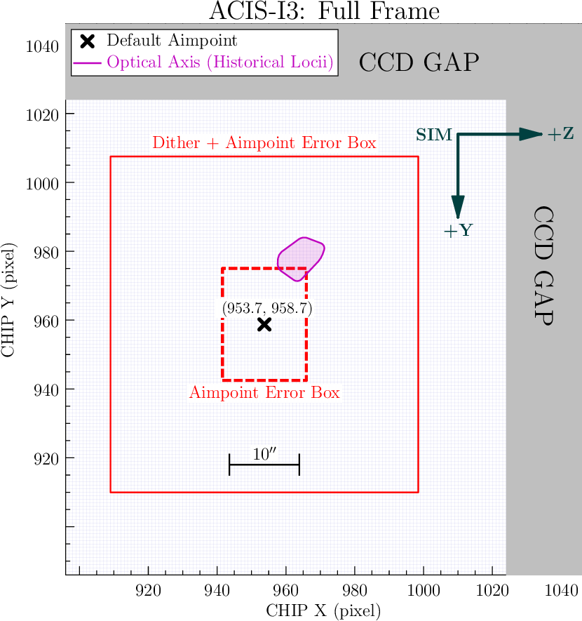
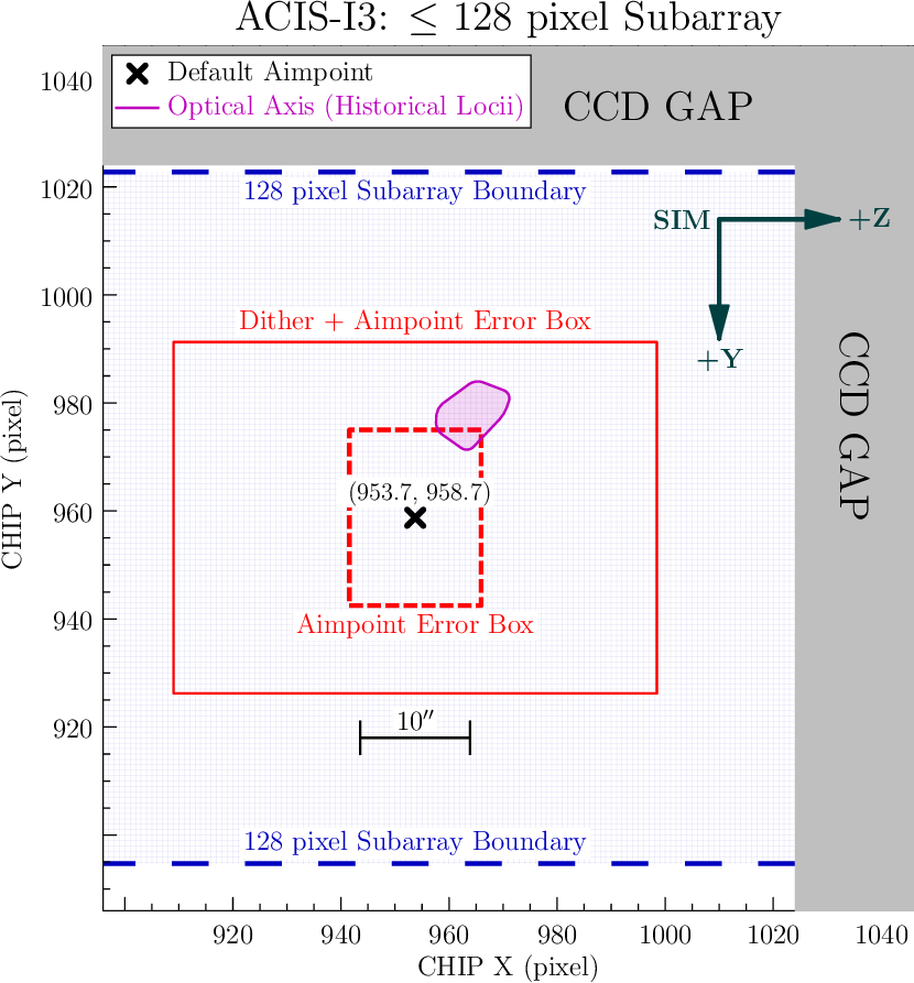
| ACIS-I | I3 | −233.587 | 961.1±3.1 | 977.2±3.1 | 953.74 | 958.74 |
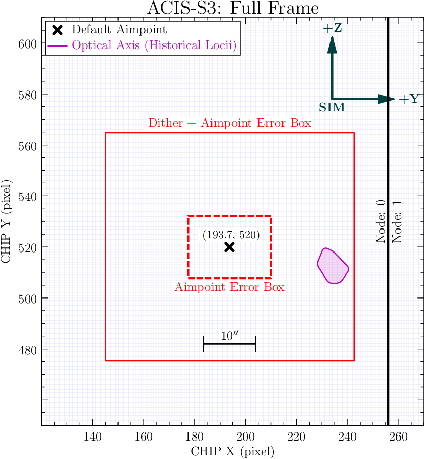
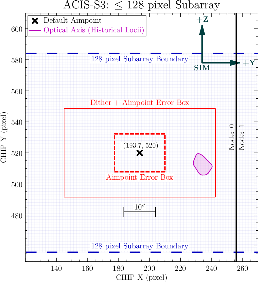
| ACIS-S | S3 | −190.143 | 234.6±3.1 | 509.1±3.1 | 193.74 | 520.00 |
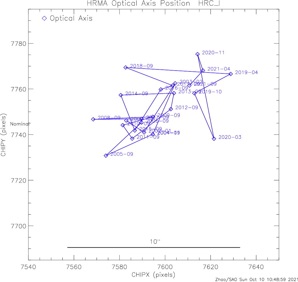
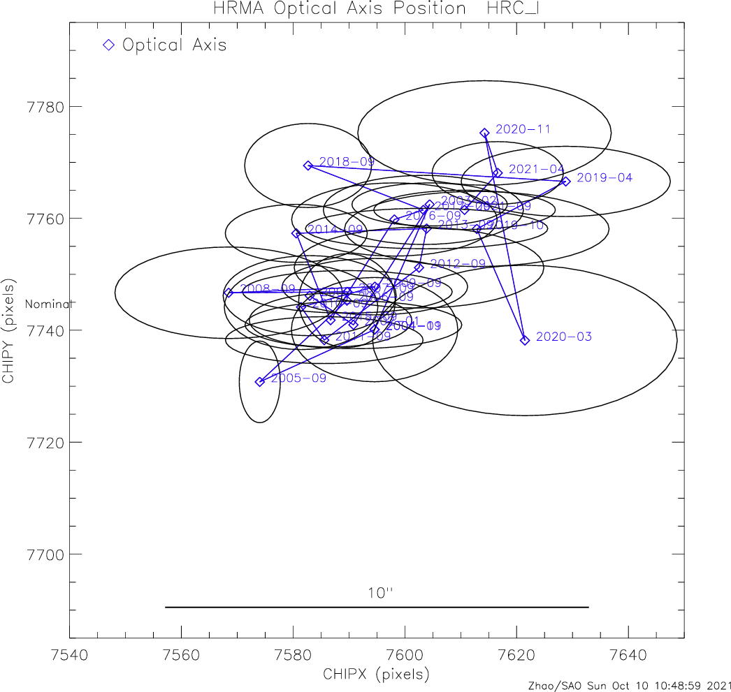
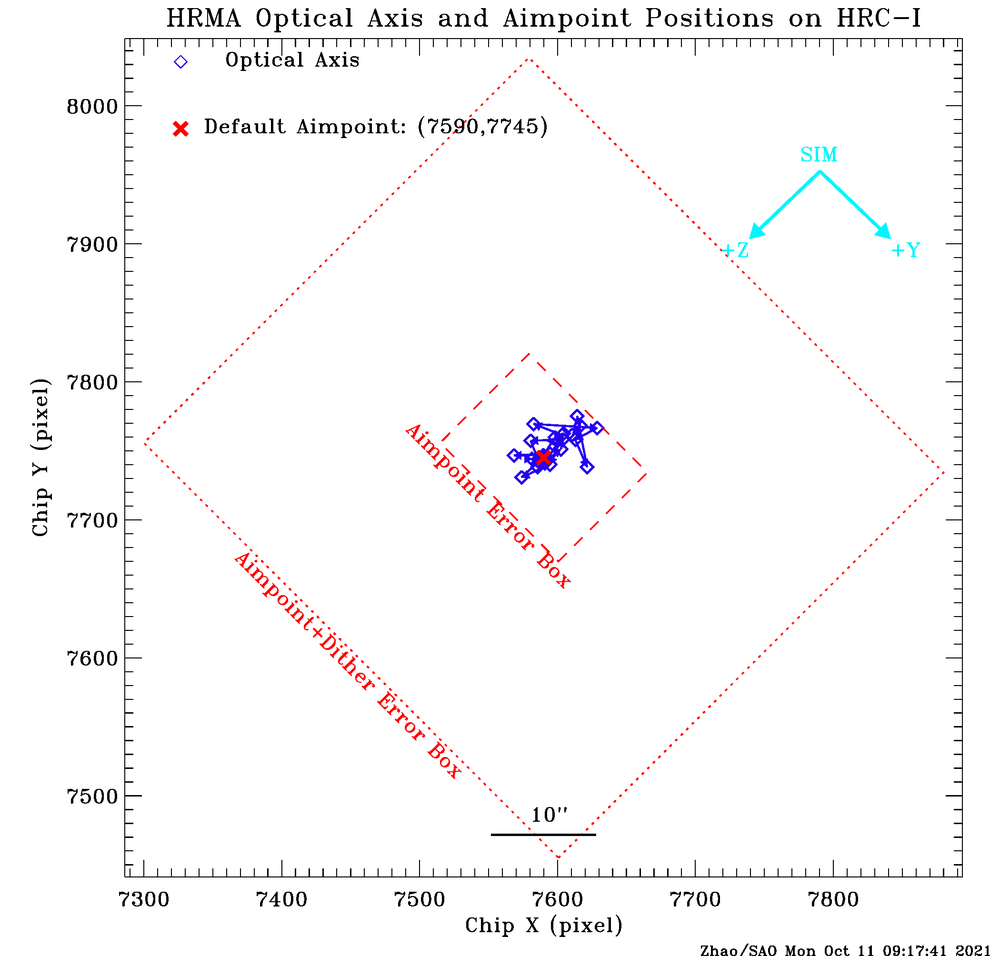
| HRC-I | 126.983 | 7610.7±15.8 | 7761.5±3.4 | 7590 | 7745 | |
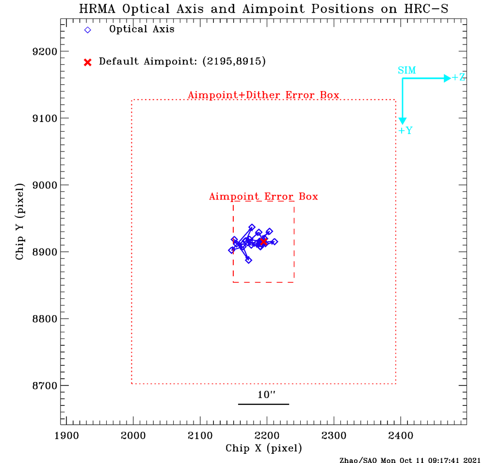
| HRC-S | S2 | 250.466 | 2163.6±11.4 | 8911.1±11.4 | 2195 | 8915 |
| Detector | Coords | Pointing Error Box | Frame Size | Total Dither Boxf | ||
| [′′] | [pixel] | [′′] | [pixel] | |||
| ACIS-I | Chip X,Y | 12" × 16" | 24.4 × 32.5 | Full | 44" × 48" | 89.44 × 97.56 |
| Sub > 128 | ||||||
| Sub ≤ 128 | 44′′×32′′ | 89.44×65 | ||||
| ACIS-S | Chip X,Y | 16" × 12" | 32.5 × 24.4 | Full | 48" × 44" | 97.56 × 89.44 |
| Sub > 128 | ||||||
| Sub ≤ 128 | 48′′×28′′ | 97.56×56.9 | ||||
| HRC-I | SIM Y,Z | 16′′×12′′ | 121.4×91.1 | Full | 56′′×52′′ | 425.0×394.7 |
| HRC-S | Chip X,Y | 12′′×16′′ | 91.1×121.4 | Full | 52′′×56′′ | 394.7×425.0 |
| f Includes pointing error | ||||||
| PREVIOUS | INDEX | NEXT |