Derived Fields

What are Derived Fields?

In the Loading Data section we already discussed the concept of fields and field specifications. For example, if we have the following Dataset:

# DON'T USE THIS LINE IF YOU ARE RUNNING IN THE IPYTHON COMMAND-LINE CONSOLE
%matplotlib inline

import acispy
msids = ["1dp28avo","1dpicacu","1deicacu","1pin1at","1pdeaat"]
ds = acispy.EngArchiveData("2015:001", "2015:030", msids, stat=None)

Then we have seven fields loaded into the Dataset, five MSIDs and two commanded states. We can look at those using the field_list attribute of the Dataset:

ds.field_list

[('msids', '1dp28avo'),
 ('msids', '1dpicacu'),
 ('msids', '1deicacu'),
 ('msids', '1pin1at'),
 ('msids', '1pdeaat'),
 ('states', 'datestart'),
 ('states', 'datestop'),
 ('states', 'tstart'),
 ('states', 'tstop'),
 ('states', 'ccd_count'),
 ('states', 'clocking'),
 ('states', 'dec'),
 ('states', 'dither'),
 ('states', 'fep_count'),
 ('states', 'hetg'),
 ('states', 'letg'),
 ('states', 'obsid'),
 ('states', 'off_nom_roll'),
 ('states', 'pcad_mode'),
 ('states', 'pitch'),
 ('states', 'power_cmd'),
 ('states', 'q1'),
 ('states', 'q2'),
 ('states', 'q3'),
 ('states', 'q4'),
 ('states', 'ra'),
 ('states', 'roll'),
 ('states', 'si_mode'),
 ('states', 'simfa_pos'),
 ('states', 'simpos'),
 ('states', 'targ_q1'),
 ('states', 'targ_q2'),
 ('states', 'targ_q3'),
 ('states', 'targ_q4'),
 ('states', 'vid_board'),
 ('states', 'trans_keys')]

So, for example, ('msids', '1dp28avo') is a “field specification” for the field itself which may be accessed in a dict-like manner:

print(ds['msids', '1dp28avo'])

[27.048 27.048 26.91  ... 27.186 27.186 27.462] V

Because the name '1dp28avo' is unique in this Dataset, we can also just get the array by simply doing:

print(ds['1dp28avo'])

[27.048 27.048 26.91  ... 27.186 27.186 27.462] V

But what if you wanted to create new fields from combinations of these fields, say, by adding two fields, or multiplying, or some other transformation. That is the purpose of a “derived field”, which has the same status as the other fields and can be accessed and plotted in the same way. ACISpy comes with some derived fields pre-defined, which can be shown using the derived_field_list of the Dataset:

ds.derived_field_list

[('states', 'grating'), ('states', 'instrument')]

In this section, we’ll show how to create your own derived fields in various ways.

Making Your Own Derived Field

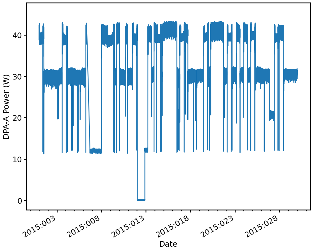
You can make your own derived field from a combination of fields that already exist, whether from raw data, another derived field, or combinations of both. In this example, we’ll show how to make a derived field. For simplicity, we’ll create a derived field that already exists, ("msids", "dpa_a_power").

First, we need to define the function that tells us what the field is:

def _dpaa_power(ds):
    return (ds["msids", "1dp28avo"]*ds["msids", "1dpicacu"]).to("W")

What we see here is that the DPA-A power is just the multiplication of ("msids", "1dp28avo") and ("msids", "1dpicacu"). This field definition simply multiplies the to and makes sure that the product is in units of Watts by calling the .to() method. Field defintion functions must take a DataContainer as their only argument. We next have to define several other things about the field:

ftype = "msids" # The type of field, since they are both MSIDs we'll keep it
fname = "my_dpa_power" # The name of the field
function = _dpaa_power # The function definition for the field
units = "W" # The units of the field
display_name = "DPA-A Power" # Optional, it controls how the field is displayed in plots

Now we can call the add_derived_field() method to set this field up:

ds.add_derived_field(ftype, fname, function, units, display_name=display_name)

We can use this field now just like any other, e.g. by examining the data:

print(ds["my_dpa_power"])

[38.792244 42.343643 39.681484 ... 31.30196  30.752804 31.342379] W

and plotting it up:

dp = acispy.DatePlot(ds, "my_dpa_power")

Mapping a State Field to a MSID’s Times

For some functions (such as PhasePlot), it may be handy to re-interpolate a state field to the times of a MSID. To do this, the DataContainer.map_state_to_msid() method is supplied to create a derived field of this kind. The optional argument ftype specifies which field type (e.g., 'msids', 'model', 'model0') to use.

ds.map_state_to_msid("pitch", "1pdeaat", ftype='msids')
print(ds["msids","pitch"])

[146.38084924 146.38084924 146.38084924 ... 131.94330066 131.94330066
 131.94330066] deg

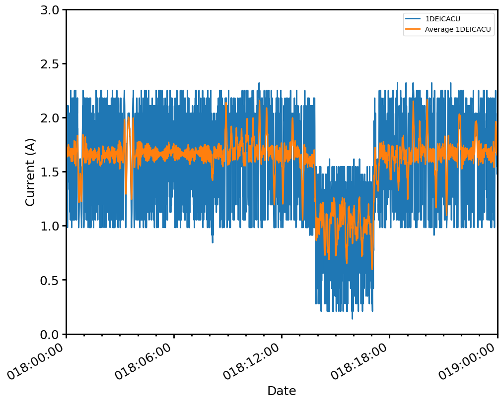
Making an Averaged Field

Some fields are particularly noisy, such as currents. For these fields, it may be helpful to examine the running or moving average of a field over time rather than its raw values. The method add_averaged_field() of the DataContainer may be used for this. To make an average field, call add_averaged_field() with the field specification that you want to average, and the number of samples n that you would like to make the running average over:

ds.add_averaged_field("1deicacu", n=10) # 10 is the default

The averaged field will have the same field specification as the original field except its name will be prefixed by "avg_". We can plot both of these fields together:

dp = acispy.DatePlot(ds, ["1deicacu", "avg_1deicacu"])
dp.set_xlim("2015:018", "2015:019")
dp.set_ylim(0.0, 3.0)