Load Review

%matplotlib inline
import acispy

The ACISLoadReview object in ACISpy can be used to obtain basic information about a particular load from the ACIS perspective. It parses the ACIS-LoadReview.txt file associated with the load, and also loads the data for the thermal models, commanded states, and telemetry data for those temperatures.

To access a particular load, simply generate a ACISLoadReview object by passing in the name of the load:

lr = acispy.ACISLoadReview("AUG0717")

acispy: [INFO     ] 2022-01-06 21:49:17,654 Reading model data from the AUG0717A load.
acispy: [WARNING  ] 2022-01-06 21:49:20,036 Could not find the model page for 'tmp_fep1_mong'. Skipping.
acispy: [WARNING  ] 2022-01-06 21:49:20,213 Could not find the model page for 'tmp_fep1_actel'. Skipping.
acispy: [WARNING  ] 2022-01-06 21:49:20,637 Could not find the model page for 'tmp_bep_pcb'. Skipping.
acispy: [WARNING  ] 2022-01-06 21:49:20,819 Could not find the earth solid angles file. Skipping.

By omitting the letter at the end, one is implying they want the latest iteration of the load, in this case, “B”. One can check this:

print(lr)

AUG0717A

You can also pass in the full name of a load iteration into the ACISLoadReview constructor, say "AUG1417A".

Accessing LoadReview Information

The ACISLoadReview object contains a number of pieces of useful information. It has attributes for the first and last times in the load:

print("First time =", lr.first_time)
print("Last time =", lr.last_time)

First time = 2017:219:10:32:43.349
Last time = 2017:226:03:30:44.065

And an attribute for the initial status of the load:

lr.start_status

{'instrument': 'HRC-S',
 'hetg_status': 'HETG-OUT',
 'letg_status': 'LETG-OUT',
 'current_obsid': '49865',
 'radmon_status': 'OORMPDS',
 'telemetry_format': 'CSELFMT2',
 'dither_status': 'ENAB'}

The ACISLoadReview object also has a number of attributes corresponding to events in the load. These attributes can be listed using the list_attributes() method:

lr.list_attributes()

obsid_change: Change of OBSID
comm_begins: Beginning of Comm
comm_ends: End of Comm
perigee: Perigee
exit_belts: Exit Radiation Belts
radmon_enable: Enable Radiation Monitor
sim_trans: SIM Translation
fmt_change: Change of Telemetry Format
letg_in: LETG Inserted
letg_out: LETG Retracted
apogee: Apogee
hetg_in: HETG Inserted
hetg_out: HETG Retracted
radmon_disable: Disable Radiation Monitor
enter_belts: Enter Radiation Belts
start_cti: Start CTI Run
end_cti: End CTI Run

Then you can access one of these attributes to examine the times of these events and/or the states associated with those times, if a state is applicable. For example, one can look at the times of OBSID changes and the new OBSID:

print("OBSID Times:")
print()
print(lr.obsid_change.times)
print()
print("OBSID States:")
print()
print (lr.obsid_change.state)

OBSID Times:

['2017:219:10:32:43.349', '2017:219:13:27:26.582', '2017:219:16:51:12.960', '2017:219:20:38:33.097', '2017:219:22:35:01.168', '2017:220:05:55:59.168', '2017:220:11:43:41.251', '2017:220:16:48:06.769', '2017:220:21:22:44.795', '2017:221:11:26:47.482', '2017:221:19:13:10.185', '2017:221:22:44:26.100', '2017:221:22:56:25.095', '2017:222:00:20:11.006', '2017:222:01:45:17.921', '2017:222:12:00:18.167', '2017:222:14:04:01.534', '2017:223:00:11:39.534', '2017:223:14:03:55.199', '2017:223:17:30:54.158', '2017:223:19:52:00.608', '2017:223:23:18:34.225', '2017:224:13:12:04.072', '2017:224:14:45:22.509', '2017:224:14:57:21.366', '2017:224:17:50:00.508', '2017:224:23:24:33.949', '2017:225:02:56:40.442', '2017:225:04:58:57.943', '2017:225:15:06:35.943', '2017:225:17:35:31.805']

OBSID States:

['49864', '49863', '49862', '49861', '19657', '19839', '19282', '19315', '19580', '19720', '19480', '49860', '49859', '49858', '49857', '49856', '20120', '20072', '19363', '18947', '19343', '19000', '19546', '49855', '49854', '49853', '49852', '49851', '17748', '19516', '19763']

Or one can print the times when a comm starts:

print("Comm Starts:")
print()
print(lr.comm_begins.times)

Comm Starts:

['2017:219:12:10:01.285', '2017:219:23:15:01.285', '2017:220:03:30:01.285', '2017:220:11:30:01.285', '2017:220:19:50:01.285', '2017:221:03:15:01.285', '2017:221:11:35:01.285', '2017:221:22:35:01.285', '2017:223:03:30:01.285', '2017:223:11:30:01.285', '2017:223:20:30:01.285', '2017:224:02:15:01.285', '2017:224:11:40:01.285', '2017:224:19:45:01.542', '2017:225:01:30:01.285', '2017:225:11:45:01.285', '2017:225:19:35:01.285', '2017:226:01:15:01.285']

Or the SIM translations and what SIM position and instrument is translated to:

print("SIM Translation Times:")
print()
print(lr.sim_trans.times)
print()
print("SIM Translation States:")
print()
print(lr.sim_trans.state)

SIM Translation Times:

['2017:219:22:32:01.168', '2017:220:05:52:59.168', '2017:220:11:43:41.251', '2017:220:21:19:44.795', '2017:221:11:23:47.482', '2017:221:22:41:26.100', '2017:222:14:01:01.534', '2017:223:14:00:55.199', '2017:224:14:42:22.509', '2017:225:04:55:57.943', '2017:225:17:32:31.805']

SIM Translation States:

[(92904, 'ACIS-I'), (-99616, 'HRC-S'), (75624, 'ACIS-S'), (92904, 'ACIS-I'), (75624, 'ACIS-S'), (-99616, 'HRC-S'), (92904, 'ACIS-I'), (75624, 'ACIS-S'), (-99616, 'HRC-S'), (75624, 'ACIS-S'), (91512, 'ACIS-I')]

The ACISLoadReview object has a Dataset object attached to it, which includes all of the thermal models and commanded states for the load in question. If the load is sufficiently far enough in the past, it also includes the temperature data corresponding to those models extracted from the engineering archive. The Dataset object in question is stored in the ds attribute of the ACISLoadReview object:

print(lr.ds["model", "1deamzt"])
print()
print(lr.ds["msids", "1deamzt"])
print()
print(lr.ds["states", "ccd_count"])

[22.54 22.62 22.66 ... 27.36 27.38 27.38] deg_C

[22.54309 22.54309 22.54309 ... 27.95636 27.95636 27.95636] deg_C

[2 2 2 ... 5 5 5]

ACISLoadReview Plotting

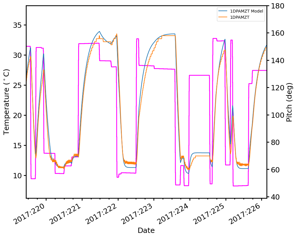
Perhaps most useful is the ability to plot thermal models and their corresponding MSID data from a load’s time period, as well as the commanded states. One can do this using the plot() method of the ACISLoadReview object. This method simply creates a DatePlot object, which one could do by hand, but has additional annotations that can also be plotted which are drawn from the load review information.

To make a basic plot of the 1DPAMZT model and data vs. time along with pitch for the whole load period:

dp = lr.plot([("model", "1dpamzt"), ("msids", "1dpamzt")], field2="pitch")

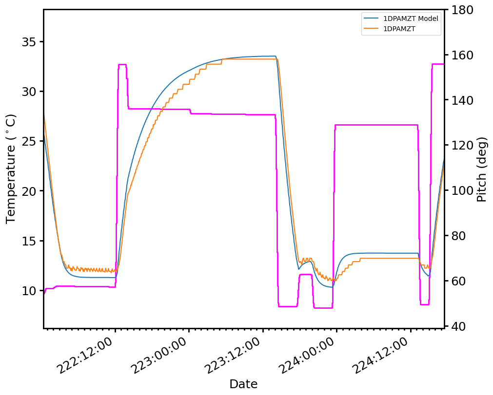
To make a plot where the plot time range is restricted to a subset within the load, use the tbegin and tend arguments:

dp = lr.plot([("model", "1dpamzt"), ("msids", "1dpamzt")], field2="pitch",
             tbegin="2017:222:00:20:30", tend="2017:224:17:30:12")

Plots made with the plot() method also accept an annotations argument, which adds useful annotations to the plot from the load review. The available annotations are:

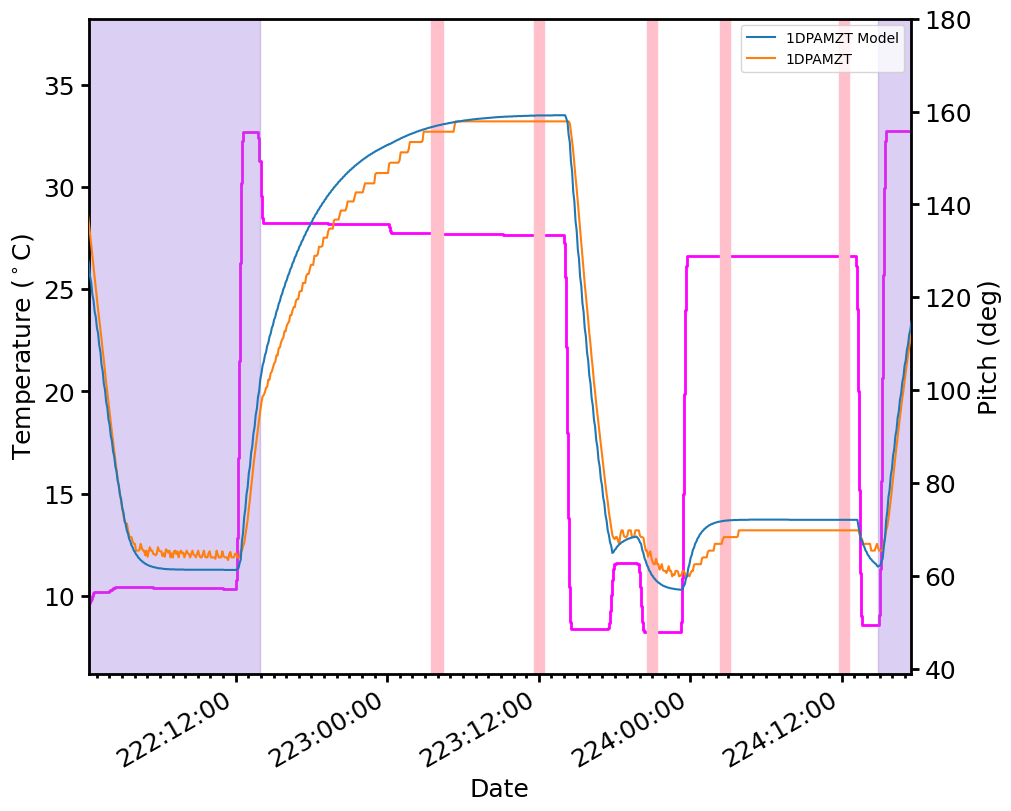
• "comms": Plot the times when we are in comm using pink bands.

• "belts": Plot the times spent in the belts using light purple bands.

• "sim_trans": Mark the times where there is a SIM translation with brown lines and lettering.

• "cti_runs": Mark the start and stop times of CTI runs with dashed green lines.

• "perigee": Mark the perigee point with a dashed blue line.

• "apogee": Mark the apogee point with a dotted blue line.

This example plots comm times from the load and times spent in the belts:

dp = lr.plot([("model", "1dpamzt"), ("msids", "1dpamzt")], field2="pitch",
             tbegin="2017:222:00:20:30", tend="2017:224:17:30:12",
             annotations=["comms", "belts"])

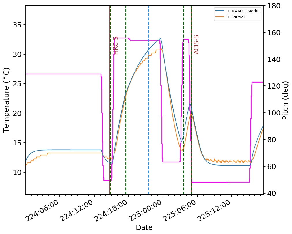
This example centers on a perigee passage and plots the sim translations, the point of perigee, and the beginnings and endings of CTI runs:

dp = lr.plot([("model", "1dpamzt"), ("msids", "1dpamzt")], field2="pitch",
             tbegin="2017:224:00:00:30", tend="2017:225:17:30:12",
             annotations=["sim_trans", "cti_runs", "perigee"])