Thermal Models#
ACISpy provides the ability to run Xija thermal models via a special class, ThermalModelRunner, which can input commanded states from a variety of sources. The really nice thing about ThermalModelRunner is that it is actually a Dataset object, so we can look at the different fields, make plots, and create derived fields.
[1]:
import acispy
import numpy as np
Basic Use of ThermalModelRunner#
If a thermal model is being run entirely within the past or another situation where kadi commanded states are fully specified, you can simply run a thermal model by specifying the MSID to be modeled and the start and stop times of the model. The initial temperature will be specified from telemetry unless one sets an initial value using the T_init keyword argument. If we want to take model “bad times” into account, we also need to set mask_bad_times=True:
[2]:
dea_model = acispy.ThermalModelRunner("1deamzt", "2020:142", "2020:150",
                                      get_msids=True, mask_bad_times=True)
acispy: [INFO ] 2025-04-17 17:21:49,657 Using model for dea from chandra_models version = 3.65
Fetching msid: aoeclips over 2020:141:23:33:58.816 to 2020:150:00:21:26.816
get_msids=True is set, so the resulting Dataset object will be populated with actual telemetry as well as model data, so that you can examine and plot both:
[3]:
print(dea_model["model","1deamzt"][:10])
print(dea_model["msids","1deamzt"][:10])
[18.04144287 17.69061317 17.34651811 17.03248643 16.73537596 16.44396592
 16.15814725 15.87781297 15.60285814 15.33317981] deg_C
[17.756287 17.506805 17.328583 17.22165  16.972137 16.687012 16.50879
 16.259277 15.902863 15.653381] deg_C
[4]:
dp = acispy.DatePlot(dea_model, [("msids", "1deamzt"), ("model", "1deamzt")], plot_bad=True)
dp
[4]:
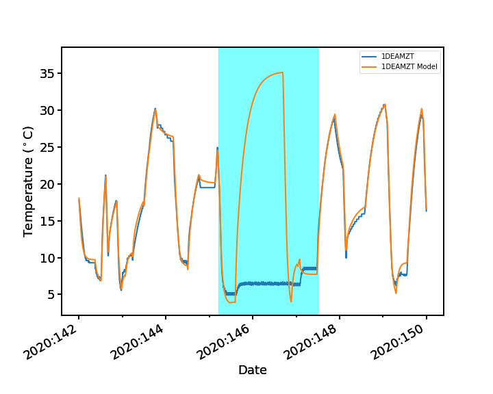
Note that for this period of time a segment of it was marked as a “bad time” in the model, and this shows up in the cyan region in the plot.
By default, model specification files will be searched for in the chandra_models package. If your model spec file is not in that package, or you want to specify a different model specification file, you can pass ThermalModelRunner a model_spec optional argument:
[5]:
dea_model2 = acispy.ThermalModelRunner("1deamzt", "2020:142", "2020:150", model_spec="dea_model_spec.json")
acispy: [INFO ] 2025-04-17 17:21:52,506 model_spec = /Users/jzuhone/Source/acispy/doc/source/dea_model_spec.json
Fetching msid: aoeclips over 2020:141:23:33:58.816 to 2020:150:00:21:26.816
Running Thermal Models Using States from Various Sources#
The ThermalModelRunner class also has various methods which one can use to run thermal models using states from various sources.
Running a Thermal Model from Commands#
You can use a set of commands (either a kadi CommandTable or list of command dicts) to run a thermal model using the from_commands method:
[6]:
from kadi import commands
# commands as a CommandTable
cmds = commands.get_cmds('2018:001:00:00:00', '2018:002:00:00:00')
psmc_model = acispy.ThermalModelRunner.from_commands("1pdeaat", cmds)
# commands as a list of dicts
dict_cmds = cmds.as_list_of_dict()
psmc_model2 = acispy.ThermalModelRunner.from_commands("1pdeaat", dict_cmds)
acispy: [INFO ] 2025-04-17 17:21:54,906 Using model for psmc from chandra_models version = 3.65
Fetching msid: aoeclips over 2018:001:02:07:50.816 to 2018:002:00:10:46.816
acispy: [INFO ] 2025-04-17 17:21:56,207 Using model for psmc from chandra_models version = 3.65
Fetching msid: aoeclips over 2018:001:02:07:50.816 to 2018:002:00:10:46.816
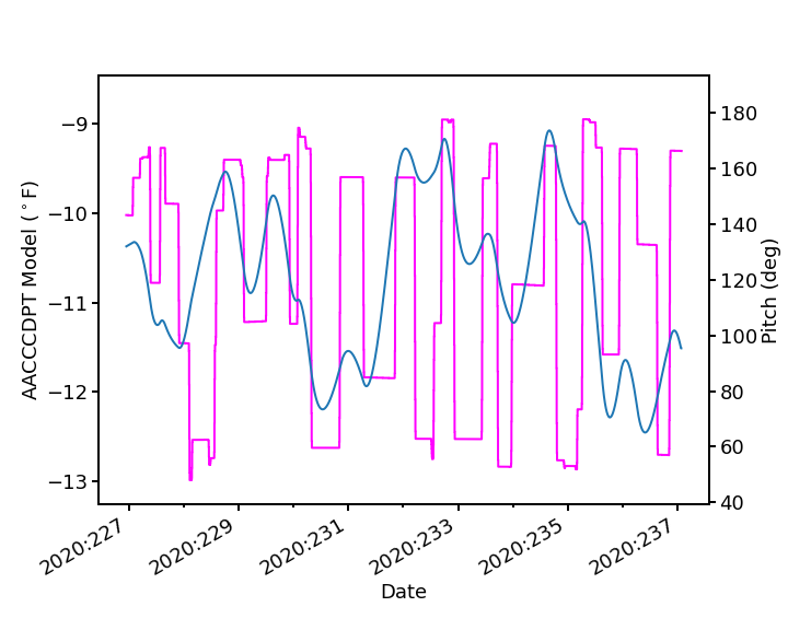
Running a Thermal Model from a Backstop File#
You can use a backstop file as input to ThermalModelRunner to generate states for a thermal model run. In this case, ThermalModelRunner will go back to the latest telemetry to determine the initial temperature (unless one is specified, see below) and construct states from that point and handle continuity between those and the commands in the backstop file appropriately. To show this, we’ll use the ACA thermal model, which requires that the initial value for the aca0 pseudonode be
specified, which we can do using the other_init keyword argument:
[7]:
tm_aca = acispy.ThermalModelRunner.from_backstop(
    "aacccdpt", "/data/acis/LoadReviews/2020/AUG1720/ofls/CR229_2202.backstop",
    other_init={"aca0": -10})
acispy: [INFO ] 2025-04-17 17:21:58,049 Using model for aca from chandra_models version = 3.65
Fetching msid: aoeclips over 2020:226:22:27:02.816 to 2020:237:01:59:26.816
[8]:
dp = acispy.DatePlot(tm_aca, ('model','aacccdpt'), field2="pitch")
dp
[8]:
Running a Thermal Model Using a states.dat File#
One can run a thermal model from a states.dat table file which would be outputted by the thermal model check scripts during a load review, using the from_states_file() method:
[9]:
dpa_model = acispy.ThermalModelRunner.from_states_file("1dpamzt", "my_states.dat")
acispy: [INFO ] 2025-04-17 17:21:58,630 Using model for dpa from chandra_models version = 3.65
Fetching msid: aoeclips over 2017:035:18:00:22.816 to 2017:051:06:00:46.816
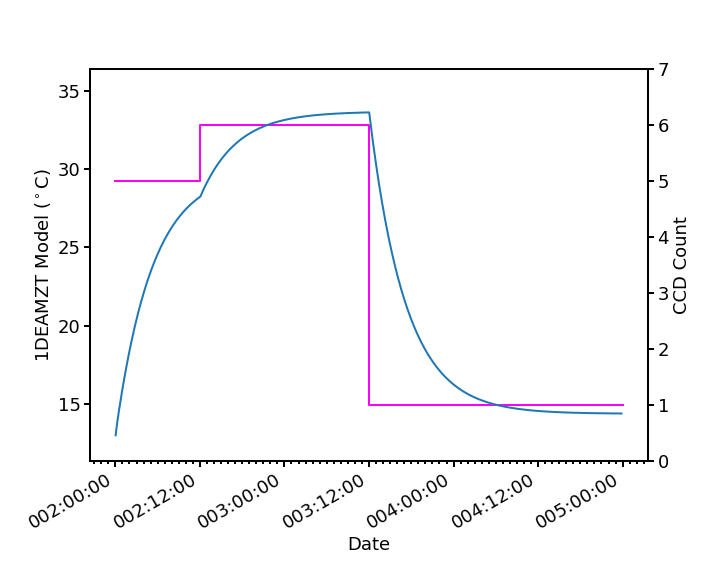
Running Thermal Models Using States Constructed By Hand#
You can create a dictionary of states completely by hand and submit them as a keyword argument to ThermalModelRunner, for running completely hypothetical thermal models. For simplicity, we’ll pick constant states except change the CCD count.
[10]:
states = {"ccd_count": np.array([5,6,1]),
          "pitch": np.array([150.0]*3),
          "fep_count": np.array([5,6,1]),
          "clocking": np.array([1]*3),
          "vid_board": np.array([1]*3),
          "off_nom_roll": np.array([0.0]*3),
          "simpos": np.array([-99616.0]*3),
          "datestart": np.array(["2015:002:00:00:00","2015:002:12:00:00","2015:003:12:00:00"]),
          "datestop": np.array(["2015:002:12:00:00","2015:003:12:00:00","2015:005:00:00:00"])}
In the previous examples, we never specified an initial temperature, but we can always do so, and must do so if we are past the end value in telemetry. This is not the case here, but we’ll set one anyway:
[11]:
T_init = 13.0 # in degrees C
Now we can pass in the states dict we created, as well as the T_init:
[12]:
dea_model = acispy.ThermalModelRunner("1deamzt", "2015:002:00:00:00",
                                      "2015:005:00:00:00", states=states, T_init=T_init)
acispy: [INFO ] 2025-04-17 17:21:58,961 Using model for dea from chandra_models version = 3.65
Fetching msid: aoeclips over 2015:001:23:34:56.816 to 2015:005:00:17:20.816
[13]:
dp = acispy.DatePlot(dea_model, ("model","1deamzt"), field2="ccd_count")
dp.set_ylim2(0,7)
dp
[13]:
We can also dump the results of the model run to disk, both the states and the model components:
[14]:
dea_model.write_model("model.dat", overwrite=True)
dea_model.write_states("states.dat", overwrite=True)
These files can be loaded in at a later date using ModelDataFromFiles.
Making Dashboard Plots#
NOTE: This functionality requires the xijafit package to be installed.#
It is possible to use the thermal model objects and the xijafit package to make dashboard plots. For this, use the make_dashboard_plots() method:
[15]:
dpa_model_long = acispy.ThermalModelRunner("1dpamzt", "2016:200", "2017:200",
                                           mask_bad_times=True, get_msids=True)
dpa_model_long.make_dashboard_plots("1dpamzt", figfile="my_dpa_dash.png")
acispy: [INFO ] 2025-04-17 17:21:59,678 Using model for dpa from chandra_models version = 3.65
Fetching msid: aoeclips over 2016:199:23:37:59.816 to 2017:200:00:17:34.816
WARNING: imaging routines will not be available,
failed to import sherpa.image.ds9_backend due to
'RuntimeErr: DS9Win unusable: Could not find xpaget on your PATH'
[15]:
<Figure size 2000x1000 with 4 Axes>
figfile sets the filename to save the dashboard plot to.
One can also use the errorplotlimits and yplotlimits arguments to set the bounds of the temperature and the errors on the plots:
[16]:
fp_model_long = acispy.ThermalModelRunner("fptemp_11", "2016:200", "2017:200",
                                          mask_bad_times=True, get_msids=True)
fp_model_long.make_dashboard_plots("fptemp_11", yplotlimits=(-120.0, -104.0),
                                   errorplotlimits=(-5.0, 5.0))
acispy: [INFO ] 2025-04-17 17:22:10,128 Using model for acisfp from chandra_models version = 3.65
Fetching msid: aoeclips over 2016:199:23:37:59.816 to 2017:200:00:17:34.816
[16]:
<Figure size 2000x1000 with 4 Axes>
Plotting Pitch and State Power Heating Values#
All thermal models have a solar heating component. To make a quick solar heating plot, use the make_solarheat_plot method, with the node that the solar heating component acts upon as the first argument.
[17]:
dpa_model_long.make_solarheat_plot("dpa0", figfile="dpa0_pitches.png")
[17]:
<Figure size 1500x1000 with 1 Axes>
Similarly, to plot the ACIS state power coefficients for a model (if present), use the make_power_plot method:
[18]:
# For the 1DEAMZT model set use_ccd_count=True
dpa_model_long.make_power_plot(figfile="acis_state_power.png", use_ccd_count=False)
[18]:
<Figure size 1000x1000 with 1 Axes>
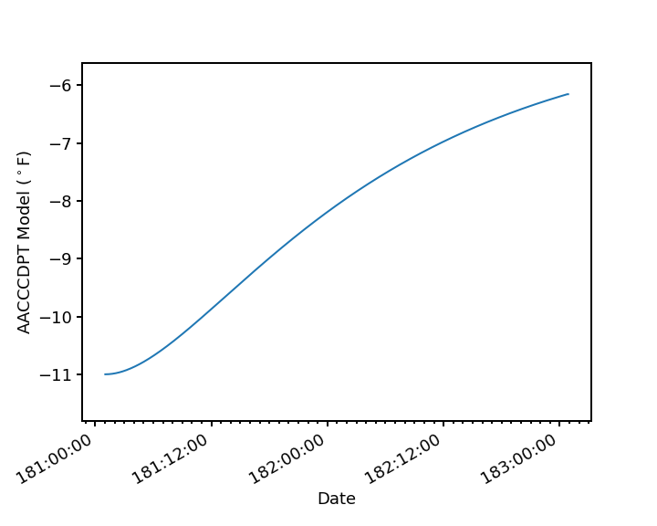
Simulating Single States#
The SimulateSingleState class is a simplified implemenation of ThermalModelRunner which assumes that the spacecraft state is constant over a period of time. This class takes the name of the temperature to simulate, a start and stop date, and a dictionary of states. It is not required to specify all states in this dictionary, but note that states not specified will be assumed to be the following:
pitch: 90 degoff_nom_roll: 0 degccd_count: 0fep_count: 0clocking: 0vid_board: 0simpos: -99616.0hetg:"RETR"letg:"RETR"dh_heater: 0q1: 1.0q2: 0.0q3: 0.0q4: 0.0
[19]:
datestart = "2019:181:01:00:00" # start time of run
datestop = "2019:183:01:00:00" # stop time of run
states = {"pitch": 70.0}
T_init = -11.0 # in degrees F
aca_m = acispy.SimulateSingleState("aacccdpt", datestart, datestop, states, T_init, other_init={"aca0": T_init})
acispy: [INFO ] 2025-04-17 17:22:16,678 Using model for aca from chandra_models version = 3.65
Fetching msid: aoeclips over 2019:181:00:35:02.816 to 2019:183:01:19:42.816
[20]:
dp = acispy.DatePlot(aca_m, "aacccdpt")
dp
[20]:
Simulating ECS Runs#
A further special case of running a single state is an ECS run, which may be performed after a safing action. The SimulateECSRun class is a limited version of SimulateSingleState which assumes that the SIM-Z position is HRC-S (-99616) and that ACIS is clocking. The goal is to predict if the temperature will hit the planning limit within the time frame of the ECS run. A start time is specified, as well as the number of hours in the ECS run (the same number of hours as specified on the
ECS CAP). Then, an attitude must be specified, which can take one of three forms:
A (pitch, off-nominal roll) combination
An attitude quaternion
The name of a load (for vehicle load ECS runs)
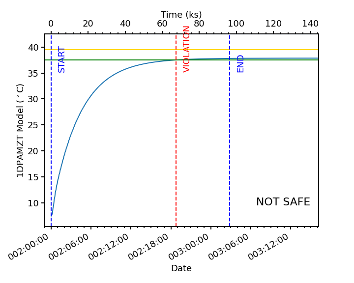
We pick a model to run (most relevant is "1dpamzt") along with a start time a length of the ECS run in hours (24 in this case), and feed the parameters into SimulateECSRun:
[21]:
datestart = "2015:002:00:00:00" # start time of run
hours = 24 # length of ECS run in hours
attitude = [173.0, 0.0] # pitch, off-nominal roll in degrees
T_init = 7.5 # in degrees C
ccd_count = 6 # number of CCDs
dpa_ecs_run = acispy.SimulateECSRun("1dpamzt", datestart, hours, T_init, attitude,
                                    ccd_count)
acispy: [INFO ] 2025-04-17 17:22:17,154 Using model for dpa from chandra_models version = 3.65
Fetching msid: aoeclips over 2015:001:23:34:56.816 to 2015:003:12:18:00.816
acispy: [INFO     ] 2025-04-17 17:22:17,373 Run Parameters
acispy: [INFO     ] 2025-04-17 17:22:17,374 --------------
acispy: [INFO     ] 2025-04-17 17:22:17,374 Modeled Temperature: 1dpamzt
acispy: [INFO     ] 2025-04-17 17:22:17,374 Start Datestring: 2015:002:00:00:00.000
acispy: [INFO     ] 2025-04-17 17:22:17,375 Length of state in hours: 24
acispy: [INFO     ] 2025-04-17 17:22:17,375 Stop Datestring: 2015:003:12:00:00.000
acispy: [INFO     ] 2025-04-17 17:22:17,375 Initial Temperature: 7.5 degrees C
acispy: [INFO     ] 2025-04-17 17:22:17,376 CCD/FEP Count: 6
acispy: [INFO     ] 2025-04-17 17:22:17,376 Pitch: 173.0
acispy: [INFO     ] 2025-04-17 17:22:17,377 Off-nominal Roll: 0.0
acispy: [INFO     ] 2025-04-17 17:22:17,377 Detector Housing Heater: OFF
acispy: [INFO     ] 2025-04-17 17:22:17,378 Model Result
acispy: [INFO     ] 2025-04-17 17:22:17,378 ------------
acispy: [INFO     ] 2025-04-17 17:22:17,380 The limit of 38.5 degrees C will be reached at 2015:002:12:47:36.816, after 46.05681599998474 ksec.
acispy: [INFO     ] 2025-04-17 17:22:17,380 The limit is reached before the end of the observation.
acispy: [WARNING  ] 2025-04-17 17:22:17,381 This observation is NOT safe from a thermal perspective.
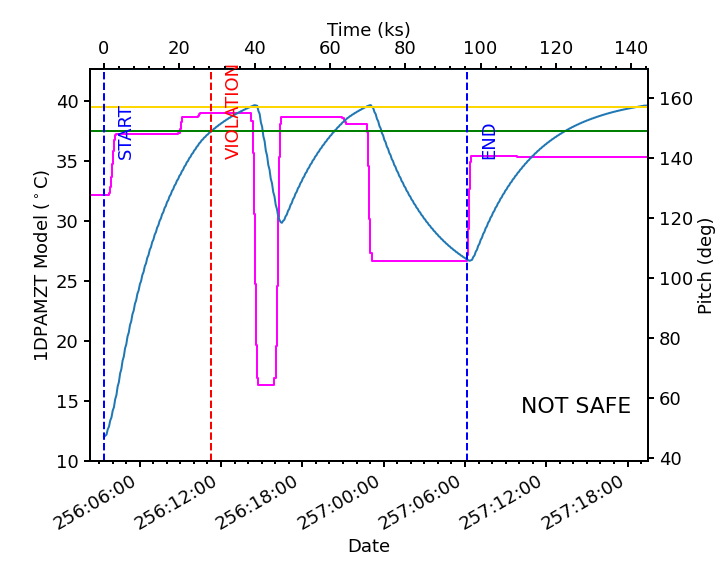
The run reports back the input parameters and the time when the limit was reached, if it was at all. We can plot the model using the plot_model() method, which shows the limit value as a dashed green line and the time at which the limit was reached as a dashed red line, as well as whether or not this was a safe ECS run:
[22]:
dpa_ecs_run.plot_model()
[22]:
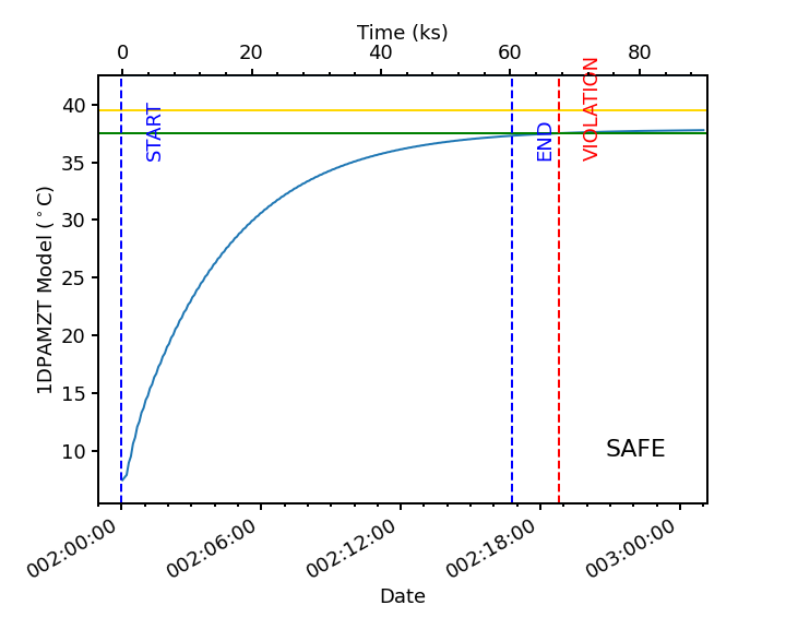
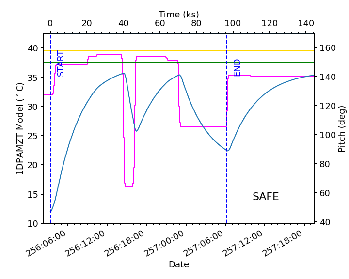
On the other hand, if the ECS run had been shorter, the limit would be reached after the ECS run, so this is safe.
[23]:
hours = 12
dpa_ecs_run = acispy.SimulateECSRun("1dpamzt", datestart, hours, T_init, attitude,
                                    ccd_count)
dpa_ecs_run.plot_model()
acispy: [INFO ] 2025-04-17 17:22:17,836 Using model for dpa from chandra_models version = 3.65
Fetching msid: aoeclips over 2015:001:23:34:56.816 to 2015:002:18:21:04.816
acispy: [INFO     ] 2025-04-17 17:22:18,010 Run Parameters
acispy: [INFO     ] 2025-04-17 17:22:18,010 --------------
acispy: [INFO     ] 2025-04-17 17:22:18,010 Modeled Temperature: 1dpamzt
acispy: [INFO     ] 2025-04-17 17:22:18,011 Start Datestring: 2015:002:00:00:00.000
acispy: [INFO     ] 2025-04-17 17:22:18,011 Length of state in hours: 12
acispy: [INFO     ] 2025-04-17 17:22:18,011 Stop Datestring: 2015:002:18:00:00.000
acispy: [INFO     ] 2025-04-17 17:22:18,011 Initial Temperature: 7.5 degrees C
acispy: [INFO     ] 2025-04-17 17:22:18,012 CCD/FEP Count: 6
acispy: [INFO     ] 2025-04-17 17:22:18,012 Pitch: 173.0
acispy: [INFO     ] 2025-04-17 17:22:18,012 Off-nominal Roll: 0.0
acispy: [INFO     ] 2025-04-17 17:22:18,012 Detector Housing Heater: OFF
acispy: [INFO     ] 2025-04-17 17:22:18,013 Model Result
acispy: [INFO     ] 2025-04-17 17:22:18,013 ------------
acispy: [INFO     ] 2025-04-17 17:22:18,014 The limit of 38.5 degrees C will be reached at 2015:002:12:47:36.816, after 46.05681599998474 ksec.
acispy: [INFO     ] 2025-04-17 17:22:18,015 The limit is reached after the end of the observation.
acispy: [INFO     ] 2025-04-17 17:22:18,015 This observation is safe from a thermal perspective.
[23]:
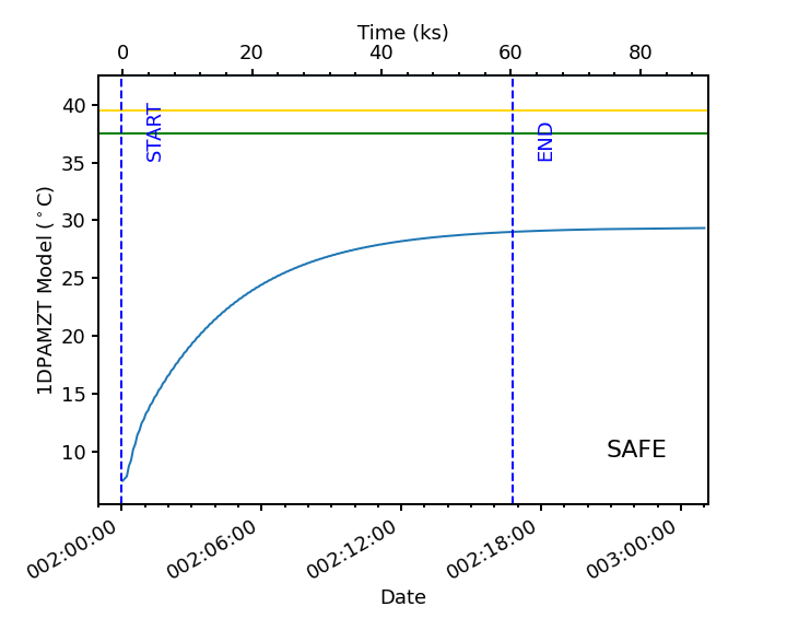
Note that for some combinations of parameters the limit may never be reached. For example, let’s knock the CCD count down to 4:
[24]:
ccd_count = 4 # only 4 CCDs
dpa_ecs_run = acispy.SimulateECSRun("1dpamzt", datestart, hours, T_init, attitude,
                                    ccd_count)
dpa_ecs_run.plot_model()
acispy: [INFO ] 2025-04-17 17:22:18,341 Using model for dpa from chandra_models version = 3.65
Fetching msid: aoeclips over 2015:001:23:34:56.816 to 2015:002:18:21:04.816
acispy: [INFO     ] 2025-04-17 17:22:18,508 Run Parameters
acispy: [INFO     ] 2025-04-17 17:22:18,508 --------------
acispy: [INFO     ] 2025-04-17 17:22:18,508 Modeled Temperature: 1dpamzt
acispy: [INFO     ] 2025-04-17 17:22:18,509 Start Datestring: 2015:002:00:00:00.000
acispy: [INFO     ] 2025-04-17 17:22:18,509 Length of state in hours: 12
acispy: [INFO     ] 2025-04-17 17:22:18,509 Stop Datestring: 2015:002:18:00:00.000
acispy: [INFO     ] 2025-04-17 17:22:18,509 Initial Temperature: 7.5 degrees C
acispy: [INFO     ] 2025-04-17 17:22:18,509 CCD/FEP Count: 4
acispy: [INFO     ] 2025-04-17 17:22:18,510 Pitch: 173.0
acispy: [INFO     ] 2025-04-17 17:22:18,510 Off-nominal Roll: 0.0
acispy: [INFO     ] 2025-04-17 17:22:18,510 Detector Housing Heater: OFF
acispy: [INFO     ] 2025-04-17 17:22:18,511 Model Result
acispy: [INFO     ] 2025-04-17 17:22:18,511 ------------
acispy: [INFO     ] 2025-04-17 17:22:18,511 The limit of 38.5 degrees C is never reached.
acispy: [INFO     ] 2025-04-17 17:22:18,511 This observation is safe from a thermal perspective.
[24]:
Simulating ECS Runs with Vehicle Loads#
If the spacecraft executed SCS-107, we may be running an ECS run while the vehicle load is still running, which means that the pitch and off-nominal roll may change during the ECS run. If this is the case, pass the name of the load to the attitude parameter. An example of an ECS run with a vehicle load that is not safe:
[25]:
datestart = "2017:256:03:20:00"
hours = 24
T_init = 12.0 # in degrees C
attitude = "vehicle" # attitude info will be take from vehicle loads
ccd_count = 6 # number of CCDs
dpa_ecs_run = acispy.SimulateECSRun("1dpamzt", datestart, hours, T_init, attitude, ccd_count)
dpa_ecs_run.plot_model()
acispy: [INFO     ] 2025-04-17 17:22:18,966 Modeling a 6-chip state concurrent with states from the following vehicle loads: {'SEP1317B', 'SEP0917C'}
acispy: [INFO     ] 2025-04-17 17:22:20,420 Using model for dpa from chandra_models version = 3.65
Fetching msid: aoeclips over 2017:256:02:54:54.816 to 2017:257:15:37:58.816
acispy: [INFO     ] 2025-04-17 17:22:20,648 Run Parameters
acispy: [INFO     ] 2025-04-17 17:22:20,648 --------------
acispy: [INFO     ] 2025-04-17 17:22:20,648 Modeled Temperature: 1dpamzt
acispy: [INFO     ] 2025-04-17 17:22:20,649 Start Datestring: 2017:256:03:20:00.000
acispy: [INFO     ] 2025-04-17 17:22:20,649 Length of state in hours: 24
acispy: [INFO     ] 2025-04-17 17:22:20,649 Stop Datestring: 2017:257:15:20:00.000
acispy: [INFO     ] 2025-04-17 17:22:20,650 Initial Temperature: 12.0 degrees C
acispy: [INFO     ] 2025-04-17 17:22:20,650 CCD/FEP Count: 6
acispy: [INFO     ] 2025-04-17 17:22:20,650 Detector Housing Heater: OFF
acispy: [INFO     ] 2025-04-17 17:22:20,651 Model Result
acispy: [INFO     ] 2025-04-17 17:22:20,651 ------------
acispy: [INFO     ] 2025-04-17 17:22:20,652 The limit of 38.5 degrees C will be reached at 2017:256:12:34:22.816, after 33.26281599998474 ksec.
acispy: [INFO     ] 2025-04-17 17:22:20,653 The limit is reached before the end of the observation.
acispy: [WARNING  ] 2025-04-17 17:22:20,653 This observation is NOT safe from a thermal perspective.
[25]:
But if we drop it down to 5 chips, it is safe:
[26]:
ccd_count = 5 # number of CCDs
dpa_ecs_run = acispy.SimulateECSRun("1dpamzt", datestart, hours, T_init, attitude, ccd_count)
dpa_ecs_run.plot_model()
acispy: [INFO     ] 2025-04-17 17:22:21,202 Modeling a 5-chip state concurrent with states from the following vehicle loads: {'SEP1317B', 'SEP0917C'}
acispy: [INFO     ] 2025-04-17 17:22:22,305 Using model for dpa from chandra_models version = 3.65
Fetching msid: aoeclips over 2017:256:02:54:54.816 to 2017:257:15:37:58.816
acispy: [INFO     ] 2025-04-17 17:22:22,501 Run Parameters
acispy: [INFO     ] 2025-04-17 17:22:22,502 --------------
acispy: [INFO     ] 2025-04-17 17:22:22,503 Modeled Temperature: 1dpamzt
acispy: [INFO     ] 2025-04-17 17:22:22,503 Start Datestring: 2017:256:03:20:00.000
acispy: [INFO     ] 2025-04-17 17:22:22,504 Length of state in hours: 24
acispy: [INFO     ] 2025-04-17 17:22:22,504 Stop Datestring: 2017:257:15:20:00.000
acispy: [INFO     ] 2025-04-17 17:22:22,504 Initial Temperature: 12.0 degrees C
acispy: [INFO     ] 2025-04-17 17:22:22,505 CCD/FEP Count: 5
acispy: [INFO     ] 2025-04-17 17:22:22,506 Detector Housing Heater: OFF
acispy: [INFO     ] 2025-04-17 17:22:22,508 Model Result
acispy: [INFO     ] 2025-04-17 17:22:22,509 ------------
acispy: [INFO     ] 2025-04-17 17:22:22,510 The limit of 38.5 degrees C is never reached.
acispy: [INFO     ] 2025-04-17 17:22:22,510 This observation is safe from a thermal perspective.
[26]:
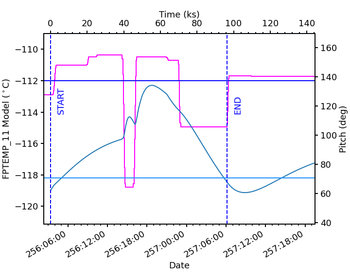
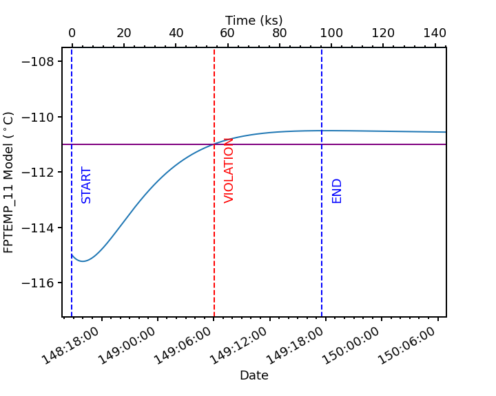
Simulating the Focal Plane Temperature for ECS Runs#
The ACIS Focal Plane (FP) temperature can also be modeled for an ECS run. This will track the amount of “cold time” for the ECS measurement. In this case, a quaternion generally should be supplied for the value of attitude, since the FP temperature can depend on the value of the Earth solid angle.
[27]:
datestart = "2020:148:14:45:00" # start time of run
hours = 24 # length of ECS run in hours
T_init = -115.0 # in degrees C
ccd_count = 4 # number of CCDs
attitude = [-0.04470333, 0.63502552, -0.67575906, 0.37160988] # attitude quaternion required

fp_ecs_run = acispy.SimulateECSRun("fptemp_11", datestart, hours, T_init, attitude, ccd_count)
fp_ecs_run.plot_model()
acispy: [INFO     ] 2025-04-17 17:22:23,173 Using model for acisfp from chandra_models version = 3.65
acispy: [WARNING  ] 2025-04-17 17:22:23,220 Using quaternions to calculate pitch and roll because both were not specified in the states.
Fetching msid: aoeclips over 2020:148:14:22:22.816 to 2020:150:03:05:26.816
acispy: [INFO     ] 2025-04-17 17:22:23,356 Run Parameters
acispy: [INFO     ] 2025-04-17 17:22:23,357 --------------
acispy: [INFO     ] 2025-04-17 17:22:23,357 Modeled Temperature: fptemp_11
acispy: [INFO     ] 2025-04-17 17:22:23,357 Start Datestring: 2020:148:14:45:00.000
acispy: [INFO     ] 2025-04-17 17:22:23,357 Length of state in hours: 24
acispy: [INFO     ] 2025-04-17 17:22:23,358 Stop Datestring: 2020:150:02:45:00.000
acispy: [INFO     ] 2025-04-17 17:22:23,358 Initial Temperature: -115.0 degrees C
acispy: [INFO     ] 2025-04-17 17:22:23,358 CCD/FEP Count: 4
acispy: [INFO     ] 2025-04-17 17:22:23,358 Quaternion: [-0.04470333, 0.63502552, -0.67575906, 0.37160988]
acispy: [INFO     ] 2025-04-17 17:22:23,359 Pitch: 155.13828486037553
acispy: [INFO     ] 2025-04-17 17:22:23,359 Off-nominal Roll: 10.637704660891393
acispy: [INFO     ] 2025-04-17 17:22:23,359 Detector Housing Heater: OFF
acispy: [INFO     ] 2025-04-17 17:22:23,360 Model Result
acispy: [INFO     ] 2025-04-17 17:22:23,360 ------------
acispy: [INFO     ] 2025-04-17 17:22:23,360 The focal plane is never cold for this ECS measurement.
acispy: [INFO     ] 2025-04-17 17:22:23,361 The limit of -86.0 degrees C is never reached.
/Users/jzuhone/mambaforge/envs/ska-dev-py312/lib/python3.12/site-packages/Ska/Matplotlib/core.py:97: UserWarning: constrained_layout not applied because axes sizes collapsed to zero.  Try making figure larger or Axes decorations smaller.
  ax.figure.canvas.draw_idle()
[27]:
This can also be done for a vehicle load as the attitude parameter:
[28]:
datestart = "2017:256:03:20:00"
hours = 24
T_init = -119.0 # in degrees C
attitude = "vehicle" # attitude info will be take from the vehicle loads
ccd_count = 6 # number of CCDs
fp_ecs_run = acispy.SimulateECSRun("fptemp_11", datestart, hours, T_init, attitude, ccd_count)
fp_ecs_run.plot_model()
acispy: [INFO     ] 2025-04-17 17:22:23,659 Modeling a 6-chip state concurrent with states from the following vehicle loads: {'SEP1317B', 'SEP0917C'}
acispy: [INFO     ] 2025-04-17 17:22:24,974 Using model for acisfp from chandra_models version = 3.65
Fetching msid: aoeclips over 2017:256:02:54:54.816 to 2017:257:15:37:58.816
acispy: [INFO     ] 2025-04-17 17:22:25,175 Run Parameters
acispy: [INFO     ] 2025-04-17 17:22:25,175 --------------
acispy: [INFO     ] 2025-04-17 17:22:25,176 Modeled Temperature: fptemp_11
acispy: [INFO     ] 2025-04-17 17:22:25,176 Start Datestring: 2017:256:03:20:00.000
acispy: [INFO     ] 2025-04-17 17:22:25,176 Length of state in hours: 24
acispy: [INFO     ] 2025-04-17 17:22:25,176 Stop Datestring: 2017:257:15:20:00.000
acispy: [INFO     ] 2025-04-17 17:22:25,176 Initial Temperature: -119.0 degrees C
acispy: [INFO     ] 2025-04-17 17:22:25,176 CCD/FEP Count: 6
acispy: [INFO     ] 2025-04-17 17:22:25,177 Detector Housing Heater: OFF
acispy: [INFO     ] 2025-04-17 17:22:25,177 Model Result
acispy: [INFO     ] 2025-04-17 17:22:25,177 ------------
acispy: [INFO     ] 2025-04-17 17:22:25,178 The focal plane is cold for 13.120000000000001 ks.
acispy: [INFO     ] 2025-04-17 17:22:25,178 The limit of -86.0 degrees C is never reached.
[28]: