Basic Usage
For this example, we will get states from a backstop file, but in theory they could come from the kadi states database, etc.
[2]:
bs_cmds = read_backstop("/data/acis/LoadReviews/2022/MAR2822/ofls/CR086_2107.backstop")
sts = states.get_states(cmds=bs_cmds, merge_identical=True)
The first example is a simple and boring one, the 1DEAMZT upper limit:
[3]:
# Create the DEALimit object
dea_limit = cl.DEALimit()
# Get the "high" limit, with states as input (though for this case they are not used)
dea_limit_line = dea_limit.get_limit_line(sts, which='high')
dea_limit_line is a LimitLine object with various useful attributes:
[4]:
print(dea_limit_line.times) # the times of the limit line
print(dea_limit_line.values) # the values of the limit line
print(dea_limit_line.reasons) # the reason for the limit at particular times
[7.64805092e+08 7.64805272e+08 7.64805276e+08 ... 7.65409624e+08
 7.65409813e+08 7.65409929e+08]
[38.5 38.5 38.5 ... 38.5 38.5 38.5]
['planning.warning.high' 'planning.warning.high' 'planning.warning.high'
 ... 'planning.warning.high' 'planning.warning.high'
 'planning.warning.high']
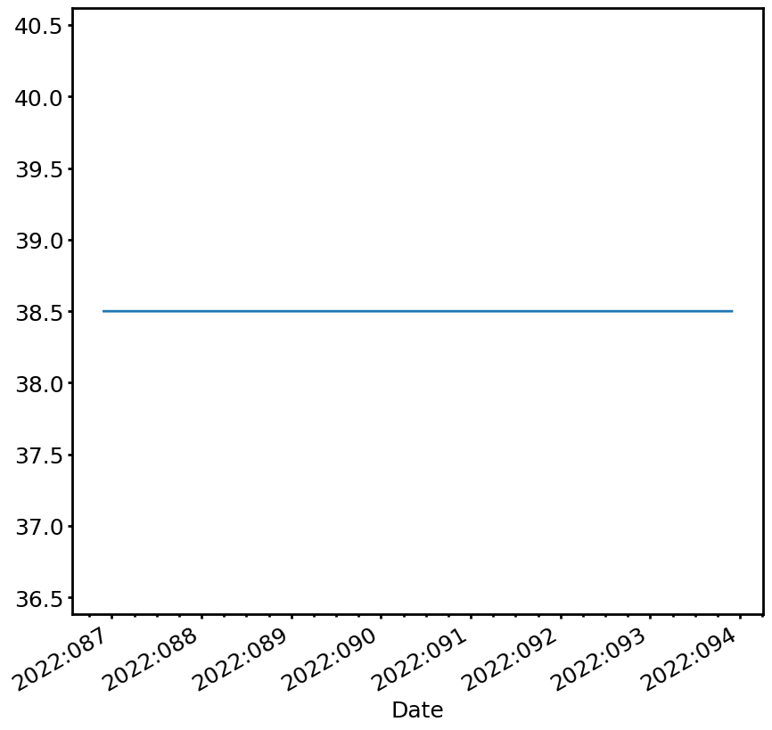
We can plot the line by itself (we’ll make this more useful below):
[5]:
fig, ax = dea_limit_line.plot(lw=2)
A more interesting limit is the zero-FEPs 1DPAMZT limit, which is a lower limit and only applies if 0 FEPs are on:
[6]:
dpa_limit = cl.DPALimit()
dpa_limit_line = dpa_limit.get_limit_line(sts, which='low')
print(dpa_limit_line.values)
print(dpa_limit_line.reasons)
[-- -- -- ... -- 13.0 13.0]
['' '' '' ... '' 'planning.caution.low' 'planning.caution.low']
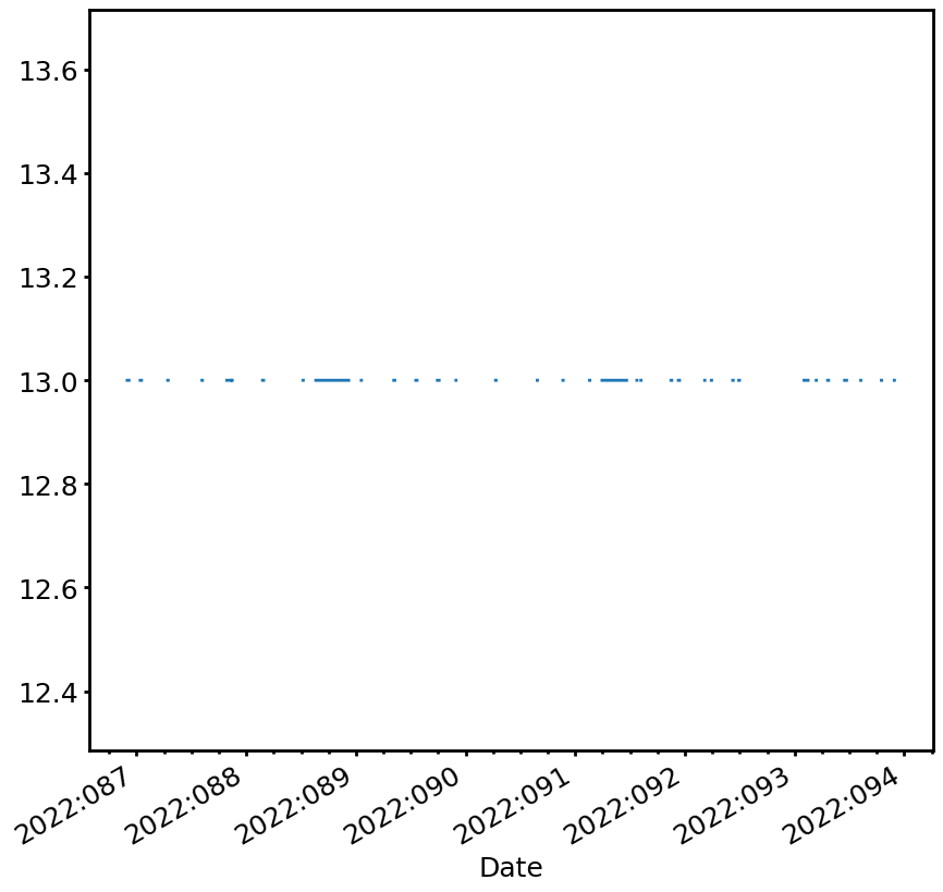
Note that in this case there is no limit at certain times. We can also see this if we plot it:
[7]:
fig, ax = dpa_limit_line.plot(lw=2)
The ACIS Focal Plane Limit
The ACIS FP limit is more complex, as it depends on a number of conditions pertaining to the schedule of observations. ACIS observations have different limits depending on which array of chips is used, whether or not there is a grating inserted, and the number of expected counts in the observation. The information about the limit values can be determined by querying the obscat, or they can be read directly from an OR list.
This limit is handled by the ACISFPLimit class. Before it can be used to create a limit line, one needs to run the ACISFPLimit.set_obs_info method, which takes as a required input a dictionary of four lists and/or NumPy arrays: obsid, start_science, stop_science, and simode. These are the observation IDs, start times, stop times, and SIMODEs of the observations in the schedule. Note that the start and stop times are defined by the times of the ACIS startScience and
stop_science commands, respectively. Note also that the SIMODE names must reflect whether or not the bias should be calculated (e.g., TE_0057AB with bias, and TE_0057A without bias). This dictionary can be constructed using any method (so long as the OBSIDs are valid). One way to make one easily is to use the determine_obsid_info helper function, which takes a states table as input (from kadi, for example) and determines the OBSIDs, their start and stop times, and the SIMODEs
from the states:
[8]:
bs_cmds2 = read_backstop("/data/acis/LoadReviews/2024/JUL1524/ofls/CR196_1802.backstop")
sts2 = states.get_states(cmds=bs_cmds2, merge_identical=True)
obs_list = cl.determine_obsid_info(sts2)
The resulting structure is very simple (showing here only a portion of the output):
[9]:
pprint(obs_list)
{'obsid': array([27229, 26521, 28164, 28810, 28926, 26952, 27424, 29481, 27427,
       28459, 28318, 27061, 29435, 28511, 29483, 25552, 27389, 26502,
       28103, 29484]),
 'simode': array(['TE_0057AB', 'TE_00958B', 'TE_00A5AB', 'TE_006E6B', 'TE_00958B',
       'TE_006E6B', 'TE_00958B', 'TE_00CBAB', 'TE_00958B', 'TE_00CE6B',
       'TE_00458B', 'TE_00866B', 'TE_006E6B', 'TE_0057AB', 'TE_00CE6B',
       'TE_005C6B', 'TE_0064CB', 'TE_0050EB', 'TE_006E6B', 'TE_006CCB'],
      dtype='<U9'),
 'start_science': array(['2024:197:03:49:03.971', '2024:197:15:00:56.776',
       '2024:197:20:58:33.359', '2024:198:04:17:39.568',
       '2024:198:06:27:15.953', '2024:198:21:00:34.546',
       '2024:199:19:43:42.398', '2024:200:06:09:49.079',
       '2024:200:12:11:03.445', '2024:200:22:34:35.340',
       '2024:201:04:58:07.460', '2024:201:11:44:16.083',
       '2024:201:20:13:46.103', '2024:202:11:39:09.836',
       '2024:202:16:21:09.077', '2024:202:19:37:50.474',
       '2024:202:21:35:03.190', '2024:203:04:21:20.254',
       '2024:203:12:58:47.215', '2024:203:18:18:10.891'], dtype='<U21'),
 'stop_science': array(['2024:197:14:50:15.971', '2024:197:20:37:54.776',
       '2024:198:00:21:07.359', '2024:198:06:13:17.568',
       '2024:198:20:43:34.953', '2024:199:08:58:02.998',
       '2024:200:05:47:40.398', '2024:200:11:56:19.079',
       '2024:200:22:15:01.445', '2024:201:04:21:45.340',
       '2024:201:06:44:05.460', '2024:201:20:08:14.083',
       '2024:201:23:52:49.846', '2024:202:16:05:21.836',
       '2024:202:19:21:39.077', '2024:202:21:05:24.474',
       '2024:202:23:21:02.190', '2024:203:12:45:18.254',
       '2024:203:18:02:45.215', '2024:203:22:48:48.891'], dtype='<U21')}
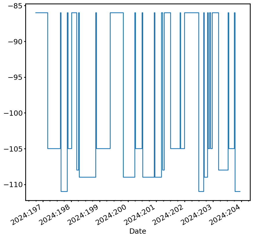
With this obs_list in hand, one can determine the ACIS FP limit line in a very similar manner to the other limits:
[10]:
acisfp_limit = cl.ACISFPLimit()
acisfp_limit.set_obs_info(obs_list)
fp_limit_line = acisfp_limit.get_limit_line(sts2)
fig, ax = fp_limit_line.plot(lw=2)

By default, the limit values for the different observations are determined by an obscat query. However, if an OR list is available, the limit values can be read directly from it like so:
[11]:
acisfp_limit = cl.ACISFPLimit()
acisfp_limit.set_obs_info(
    obs_list,
    orlist="/data/acis/LoadReviews/2024/JUL1524/ofls/mps/or/JUL1524_A.or"
)
fp_limit_line = acisfp_limit.get_limit_line(sts2)
fig, ax = fp_limit_line.plot(lw=2)
Note that the two limit lines obtained by either method are identical, as they should be.
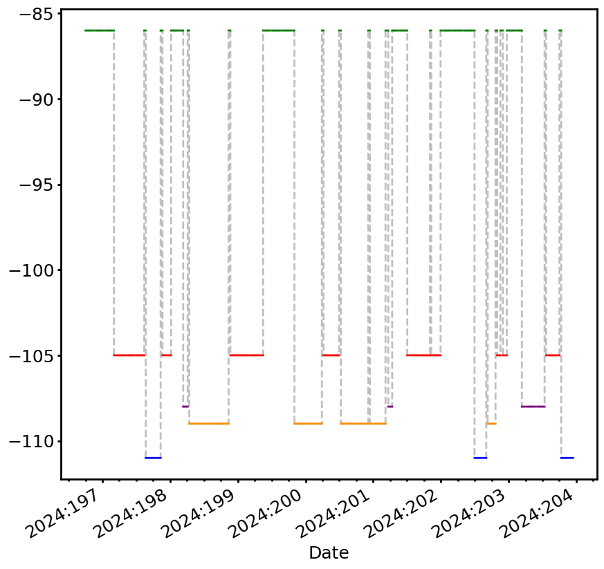
If you want to plot the limit so that the different limit reasons have different colors, you can set use_colors=True:
[12]:
fig, ax = fp_limit_line.plot(lw=2, use_colors=True)
Running with Models and Checking for Violations
Now we show an example where we run a thermal model, check the limit against it, and see if there are violations. We’ll use the 1DPAMZT model:
[13]:
dpa_json = get_xija_model_spec("dpa")[0]
tm_dpa = xija.XijaModel("dpa", sts["datestart"][0], sts["datestop"][-1],
                        model_spec=dpa_json, cmd_states=sts)
tm_dpa.comp["dpa0"].set_data(10.0)
tm_dpa.make()
tm_dpa.calc()
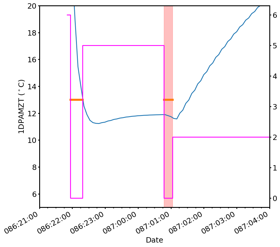
We feed the states and the times from the model, and then check the violations using the check_violations method of the LimitLine object. In this case, we’ll check the low-temperature limit:
[14]:
dpa_limit_line = dpa_limit.get_limit_line(sts, which='low')
viols = dpa_limit_line.check_violations(tm_dpa)
Two violations were found:
[15]:
pprint(viols)
[{'datestart': '2022:087:00:47:01.462',
  'datestop': '2022:087:01:02:45.085',
  'duration': 0.94362299990654,
  'extemp': 11.671603014252552,
  'limit': 13.0,
  'reason': 'planning.caution.low'},
 {'datestart': '2022:092:05:47:13.724',
  'datestop': '2022:092:05:49:46.227',
  'duration': 0.15250300002098083,
  'extemp': 12.899406305964627,
  'limit': 13.0,
  'reason': 'planning.caution.low'}]
We can double-check the first one by eye by plotting the model, the FEP count, and the limit line. We can also use the helper function plot_viols to plot bands where the violations occur:
[16]:
fig, ax = plt.subplots(figsize=(10,10))
ax2 = ax.twinx()
x = pointpair(CxoTime(sts["datestart"]).plot_date,
              CxoTime(sts["datestop"]).plot_date)
y = pointpair(sts["fep_count"])
ax2.plot(x, y, lw=2, color='magenta', drawstyle='steps')
ax.plot(CxoTime(tm_dpa.times).plot_date, tm_dpa.comp["1dpamzt"].mvals, lw=2)
dpa_limit_line.plot(lw=5, fig_ax=(fig, ax), color="C1")
ax.set_xlim(CxoTime("2022:086:21:00:00").plot_date,
            CxoTime("2022:087:04:00:00").plot_date)
ax.set_ylim(5, 20)
ax.set_ylabel("1DPAMZT ($^\circ$C)")
cl.plot_viols(ax, viols, alpha=0.25)
We can try the same thing for the focal plane model:
[17]:
acisfp_json = get_xija_model_spec("acisfp")[0]
tm = xija.XijaModel("acisfp", sts2["datestart"][0], sts2["datestop"][-1],
                    model_spec=acisfp_json, cmd_states=sts2)
tm.make()
tm.calc()

obs_list = cl.determine_obsid_info(sts2)
acisfp_limit = cl.ACISFPLimit(margin=0.0)
acisfp_limit.set_obs_info(obs_list)
fp_limit_line = acisfp_limit.get_limit_line(sts, which='high')
viols = fp_limit_line.check_violations(tm)
In this case, many violations were found:
[18]:
pprint(viols)
[{'datestart': '2024:197:19:49:50.816',
  'datestop': '2024:197:21:17:18.816',
  'duration': 5.248,
  'extemp': -108.6902292750602,
  'limit': -111.0,
  'obsid': 26521,
  'reason': 'planning.data_quality.high.acis_0'},
 {'datestart': '2024:199:09:33:02.816',
  'datestop': '2024:199:17:45:02.816',
  'duration': 29.52,
  'extemp': -97.44808607595085,
  'limit': -105.0,
  'obsid': 26952,
  'reason': 'planning.data_quality.high.acis_2'},
 {'datestart': '2024:199:20:04:20.398',
  'datestop': '2024:199:20:34:30.816',
  'duration': 1.8104179999828338,
  'extemp': -108.39461728664544,
  'limit': -109.0,
  'obsid': 27424,
  'reason': 'planning.data_quality.high.grating_0'},
 {'datestart': '2024:201:23:46:46.816',
  'datestop': '2024:202:04:36:30.816',
  'duration': 17.384,
  'extemp': -104.02615300175775,
  'limit': -105.0,
  'obsid': 29435,
  'reason': 'planning.data_quality.high.acis_2'},
 {'datestart': '2024:202:06:09:26.816',
  'datestop': '2024:202:08:26:06.816',
  'duration': 8.2,
  'extemp': -100.77563409096136,
  'limit': -105.0,
  'obsid': 29435,
  'reason': 'planning.data_quality.high.acis_2'},
 {'datestart': '2024:202:19:33:02.816',
  'datestop': '2024:202:19:54:54.816',
  'duration': 1.312,
  'extemp': -108.43915469100992,
  'limit': -109.0,
  'obsid': 29483,
  'reason': 'planning.data_quality.high.grating_0'},
 {'datestart': '2024:203:12:29:50.816',
  'datestop': '2024:203:13:19:02.816',
  'duration': 2.952,
  'extemp': -107.05120046546605,
  'limit': -108.0,
  'obsid': 26502,
  'reason': 'planning.data_quality.high.acis_1'}]
We can plot some of these also:
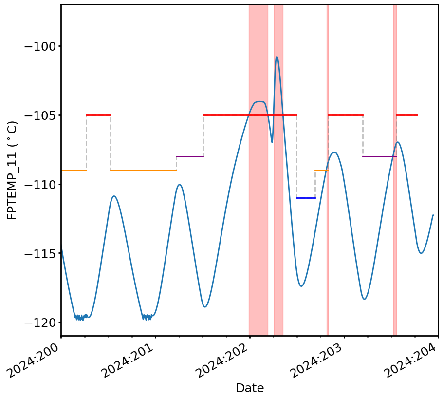
[19]:
fig, ax = plt.subplots(figsize=(10,10))
ax.plot(CxoTime(tm.times).plot_date, tm.comp["fptemp"].mvals, lw=2)
fp_limit_line.plot(lw=2, use_colors=True, fig_ax=(fig, ax))
ax.set_xlim(CxoTime("2024:200:00:00:00").plot_date,
            CxoTime("2024:204:00:00:00").plot_date)
ax.set_ylim(-121, -97)
ax.set_ylabel("FPTEMP_11 ($^\circ$C)")
cl.plot_viols(ax, viols, alpha=0.25)