Storms Command Line Tools#
Activating#
The storms command-line tools are installed into the ACIS Ops Ska Python stack.
If you are logged on as acisdude, all you need to do is issue the
command acisska and this Python stack and the tools will be loaded into
your environment.
However, if you would like activate this stack and these tools from your own user
account, add the following alias to your .bashrc if you are using the Bash
shell (or a variant):
alias acisska='eval "$(/data/acis/mambaforge/bin/conda shell.zsh hook)"; \
               export SKA=/proj/sot/ska; \
               conda activate ska'
Or, if you are a mascohist or are otherwise compelled to use the C shell or a
variant of it, add this alias to your .cshrc.user:
alias acisska 'source /data/acis/mambaforge/etc/profile.d/conda.csh; \
               setenv SKA /proj/sot/ska; \
               conda activate ska'
calc_p3_fluence#
This tool allows one to calculate the ACE P3 fluence that was saved by a safing action, compared to the amount of fluence that was actually accumulated.
usage: calc_p3_fluence [-h] radmon_enable_time return_to_science_time

positional arguments:
  radmon_enable_time   The time of radmon enable (beginning of science orbit) in YYYY:DOY:HH:MM:SS format.
  return_to_science_time
                        The time of first command in the return to science load.

options:
  -h, --help            show this help message and exit
Example 1#
[~]$ calc_p3_fluence 2024:160:01:08:34.744 2024:163:00:57:00.000
Returns:
RADMON Enable: 2024:160:01:08:34.744
Return to science: 2024:163:00:57:00.000

SCS 107 occured at 2024:160:02:29:32.127.

Potential fluence: 0.85 × 10⁹
Actual fluence: 0.00 × 10⁹
Fluence avoided: 0.85 × 10⁹
Example 2#
[~]$ calc_p3_fluence 2026:018:20:26:20.632 2026:021:15:27:09.725
Returns:
RADMON Enable: 2026:018:20:26:20.632
Return to science: 2026:021:15:27:09.725

SCS 107 occured at 2026:019:09:52:12.534.

Potential fluence: 4.26 × 10⁹
Actual fluence: 0.03 × 10⁹
Fluence avoided: 4.23 × 10⁹
make_storm_plots#
This script produces a set of plots for a storm memo of the following quantities:
ACE P3 Flux
ACE Proton Fluxes
ACE Electron Fluxes
GOES Proton Fluxes
HRC Proxy
txings Rates
txings Rates (zoomed-in)
It only takes one argument, which is the filename which contains the parameters for making the plots.
usage: make_storm_plots [-h] infile

Plot solar wind data for a given time range.

positional arguments:
  infile      The YAML file containing the parameters for plotting.

options:
  -h, --help  show this help message and exit
Example 1#
[~]$ make_storm_plots nov2025.yml
where the contents of the YAML file nov2025.yml are:
### Parameter file for storm plots

# Basename for output files
basename: "nov2025"


## Time range for data extraction

# sometime before SCS-107, and maybe before RADMON enable
start: "2025:314:00:00:00"

# sometime after return to science
stop: "2025:320:12:00:00"

## Relevant times for drawing lines

# Time of SCS-107
scs_107: "2025:315:10:58:50.000"

# Time of return to science (time of first command)
rts: "2025:318:21:52:00.000"

# These will only be present if an ECS measurement is run
#ecs_start: "2025:318:00:59:50.923"
#ecs_stop: "2025:318:21:52:00.000"

## Options to change y-axis limits for plots, otherwise sane auto-defaults are chosen
#txings_limits: [0.1, 100]
#ace_p3_limits: [2e2, 8.0e5]
#ace_p_limits: [10, 5.0e6]
#goes_limits: [6e-7, 250]
#ace_e_limits: [120, 3.0e6]
#hrc_limits: [9, 7.0e3]


## Legend position
legend_loc: "lower center"
which produces the following output:
Plotting ACE P3 Flux.
Plotting ACE Proton Flux.
Plotting ACE Electron Flux.
Plotting Goes Proton Flux.
Plotting HRC Proxy.
Plotting txings rates.
Plotting zoom-in of txings rates.
and the following plots:
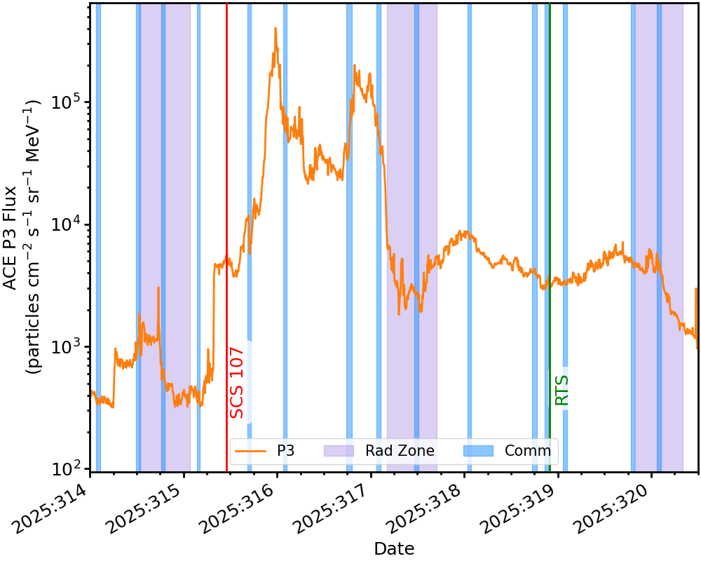
ACE P3:
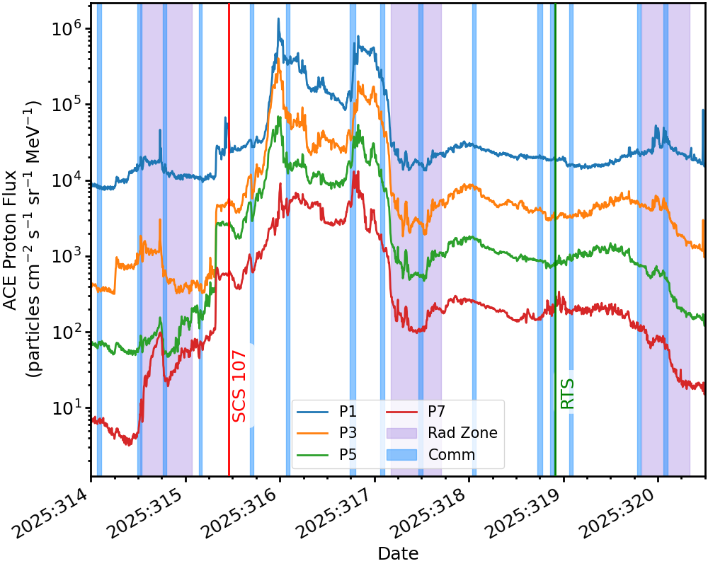
ACE Protons:
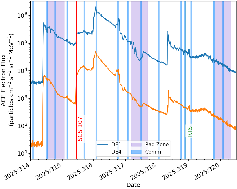
ACE Electrons:
GOES Protons:
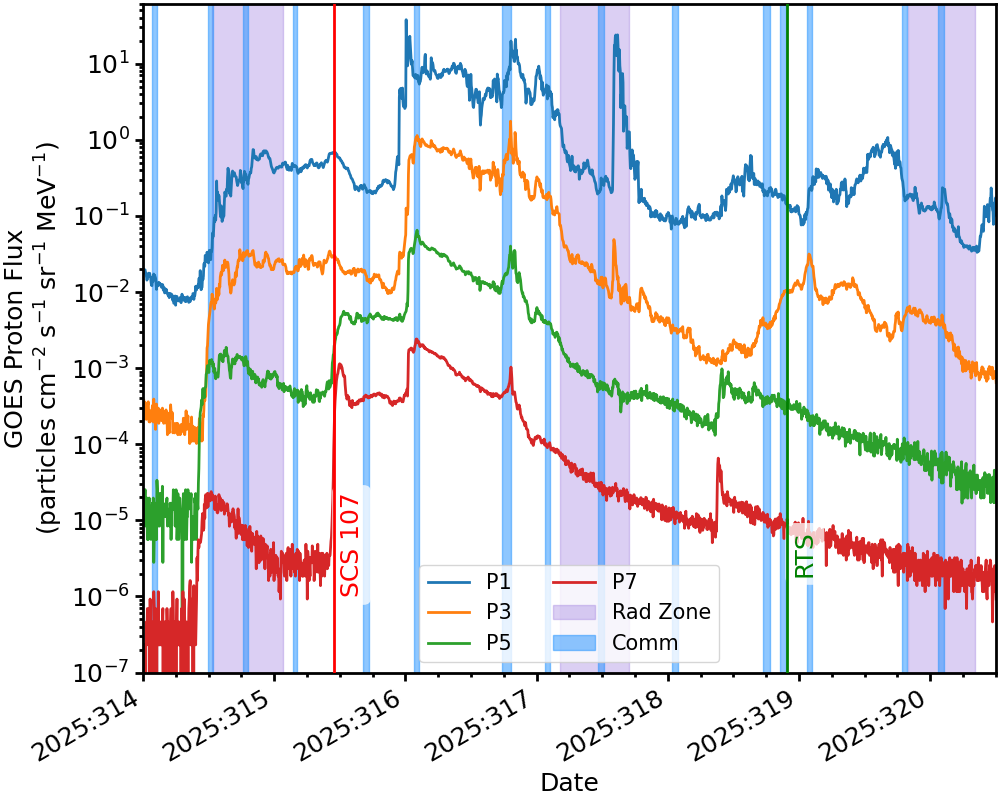
HRC Proxy:
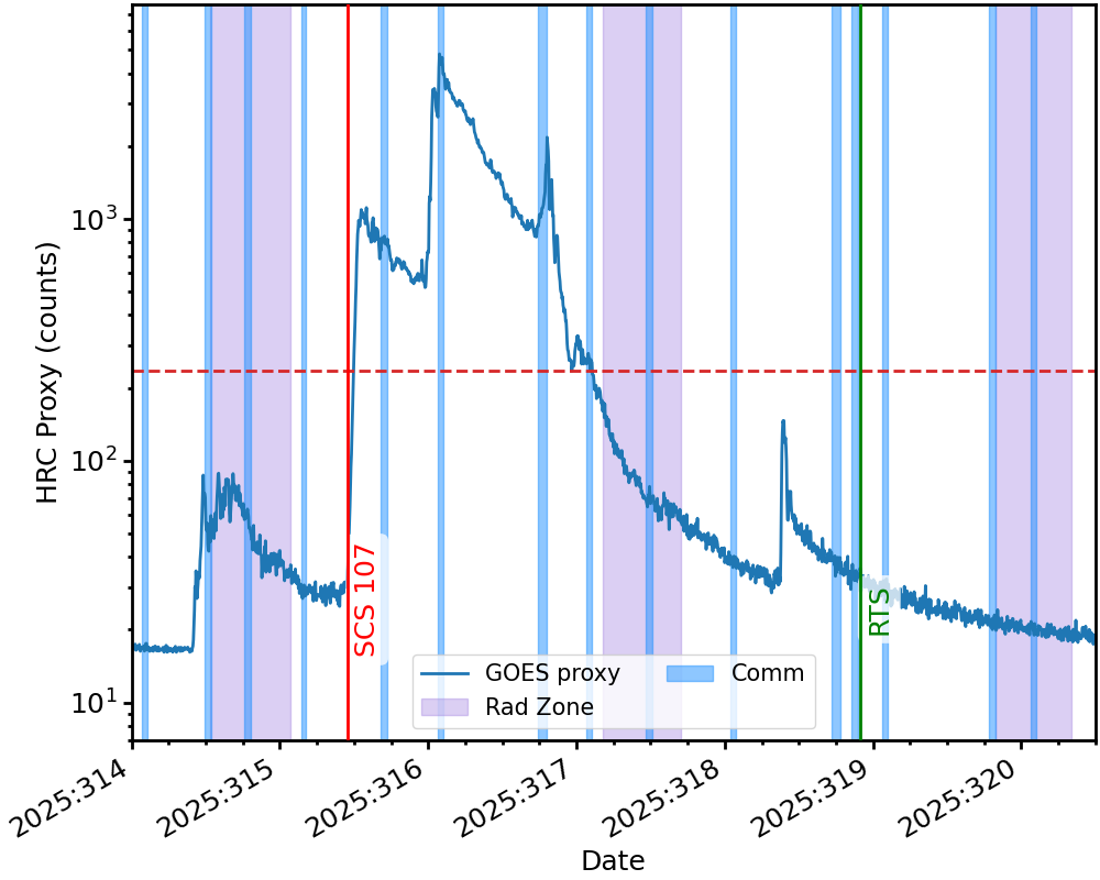
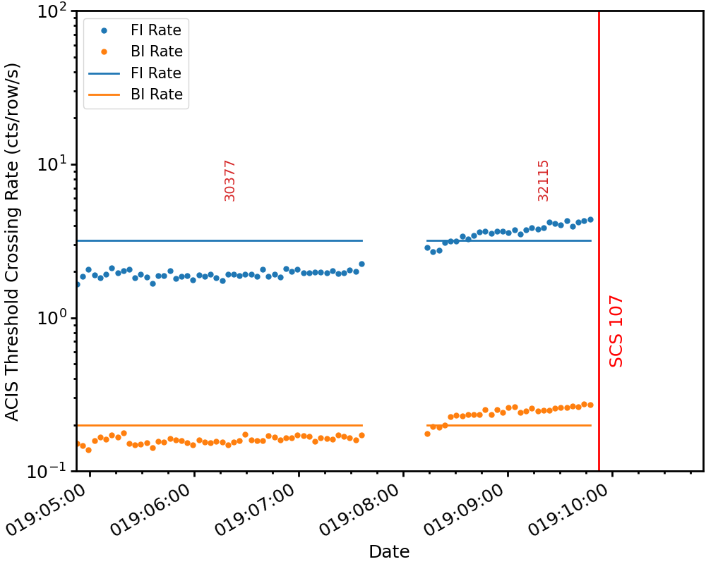
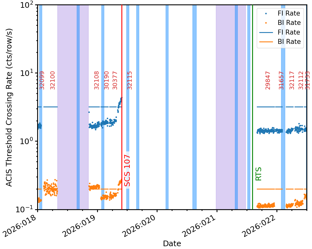
txings Rates:
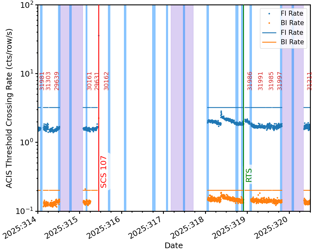
txings Rates (zoomed-in):

Example 2#
[~]$ make_storm_plots jan2026.yml
where the contents of the YAML file jan2026.yml are:
### Parameter file for storm plots

## Basename for output files
basename: "jan2026"


## Time range for data extraction

# sometime before SCS-107, and maybe before RADMON enable
start: "2026:018:00:00:00"

# sometime after return to science
stop: "2026:022:12:00:00"


## Relevant times for drawing lines

# Time of SCS-107
scs_107: "2026:019:09:52:11.046"

# Time of return to science (time of first command)
rts: "2026:021:14:12:00.000"

# These will only be present if an ECS measurement is run
#ecs_start: "2025:318:00:59:50.923"
#ecs_stop: "2025:318:21:52:00.000"


## Options to change y-axis limits for plots, otherwise sane auto-defaults are chosen
#txings_limits: [0.1, 100]
#ace_p3_limits: [2e2, 8.0e5]
#ace_p_limits: [10, 5.0e6]
#goes_limits: [6e-7, 250]
#ace_e_limits: [120, 3.0e6]
#hrc_limits: [9, 7.0e3]


## Legend position
legend_loc: "upper right"
which produces the following output:
Plotting ACE P3 Flux.
Plotting ACE Proton Flux.
Plotting ACE Electron Flux.
Plotting Goes Proton Flux.
Plotting HRC Proxy.
Plotting txings rates.
Plotting zoom-in of txings rates.
and the following plots:
ACE P3:
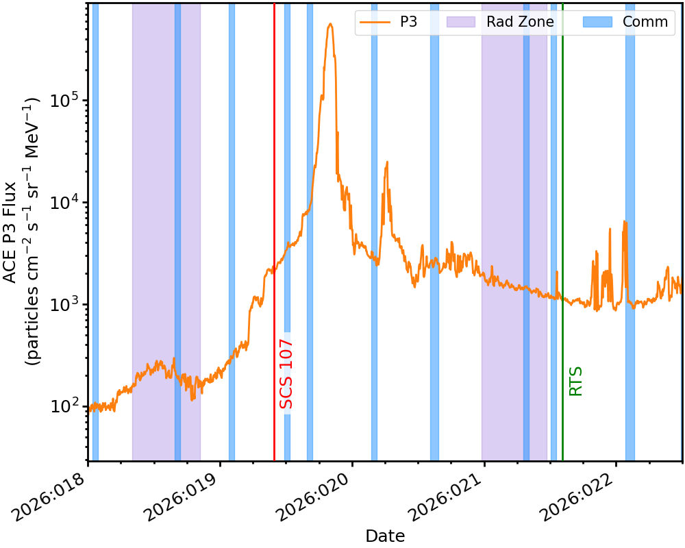
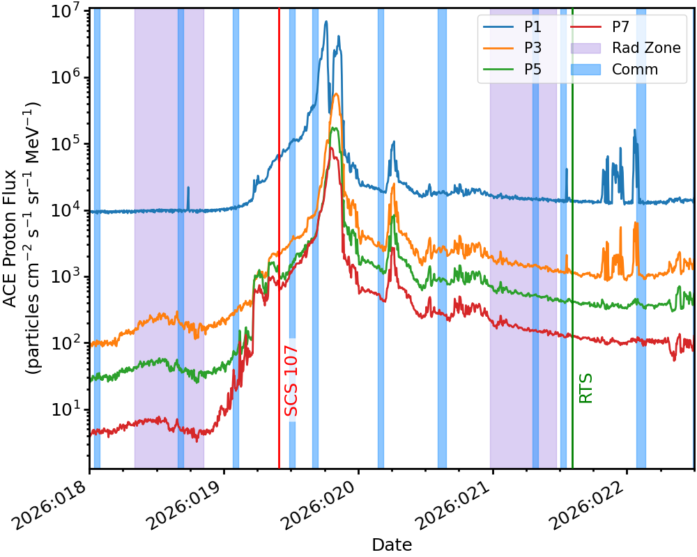
ACE Protons:
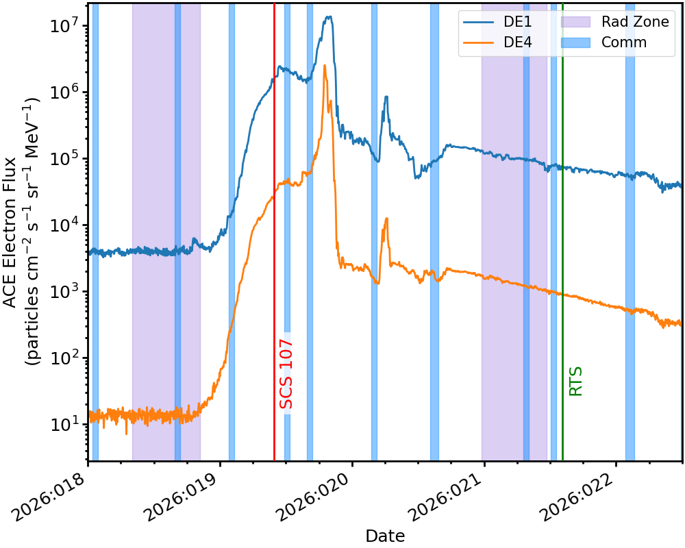
ACE Electrons:
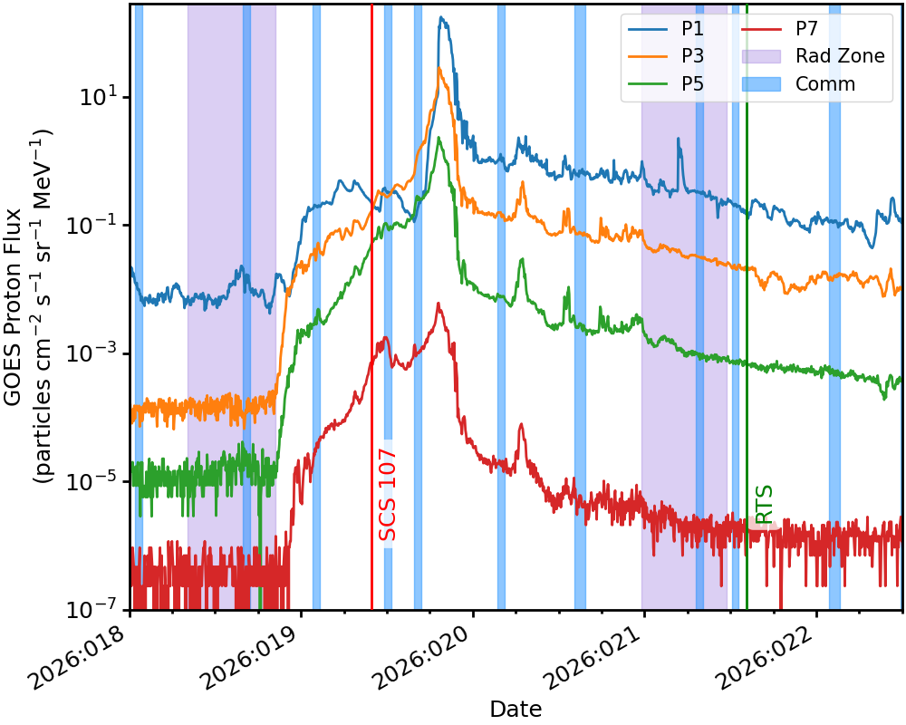
GOES Protons:
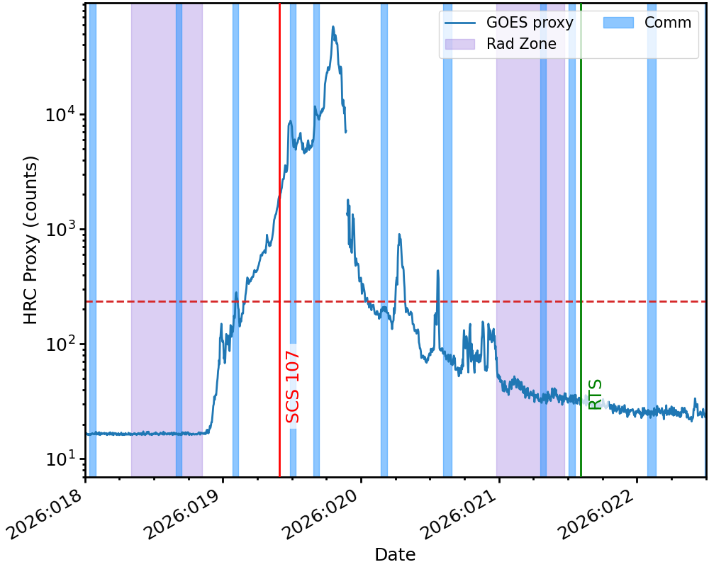
HRC Proxy:
txings Rates:
txings Rates (zoomed-in):