HRC-S flat fields were acquired at 7 energies (0.183, 0.277, 0.525, 0.852, 1.487, 4.511, 6.404 keV) in the HRC Lab prior to flight. These flats unavoidably included the UV/ion shield structure in the data. The data were binned up by 128 pixels (half-tap) for good statistics. The original flat field QE data can be found here.

HRC-S QE Uniformity was derived in the following way:
(click on figures to get larger and clearer images)

The process of deriving flatfield models from the HRC Lab data first requires the removal the complex structure of the HRC-S UV/ion shield (UVIS), as seen in Figure 1. The models for the different regions can be found here.

Figure 1: Structure of HRC-S UVIS (different regions require different transmission models).

The UVIS was divided out of the HRC-S flat fields, leaving bare MCP QEs at 7 energies. These were all normalized to the HRC-S nominal aimpoint. As an example, Figure 2 shows the central plate surface at C-K produced after removing the UVIS. (the departures at the edges are artifacts of division and are ignored for surface modeling).

Figure 2: Bare MCP QE surface of central plate at C-K (UVIS removed).

In order to correct for the spatial non-uniformities of the HRC-S QE, polynomial curves were fit to the nominal LETG dispersion line on the HRC-S (a rectangular strip located within the extraction region of the LETG). Thus, the fit polynomial curves are models of QE spatial uniformity along the dispersion axis at specific energies (ie. QEU(x,E=0.277 keV) for C-K, etc.). Figure 3 below shows the nominal LETG dispersion strips with fit polynomial curves for the full data set of 7 energies acquired on the center plate, and 4 energies acquired on each of the wing plates.

Figure 3: Polynomial Fits to QE FlatFields at 7 Energies
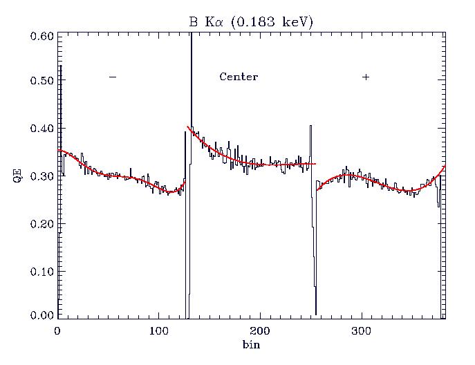
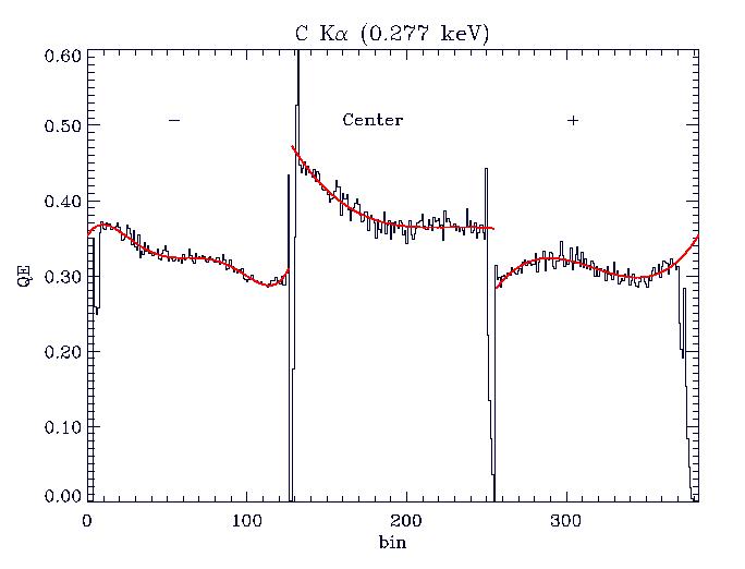
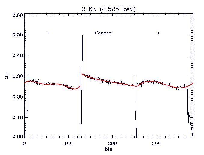
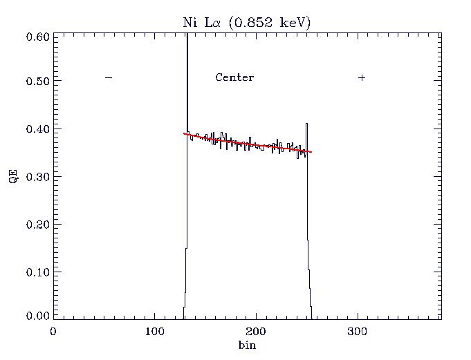
B K - 0.183 keV	C K - 0.277 keV	O K - 0.525 keV	Ni L - 0.852 keV
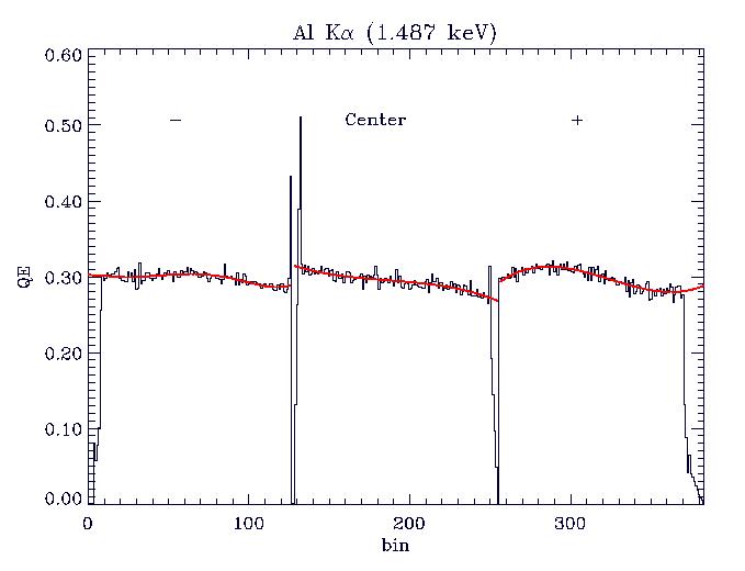
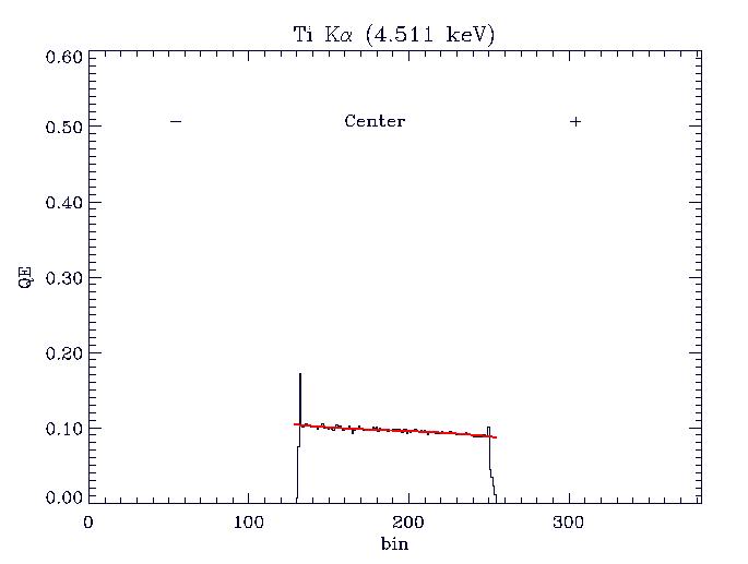
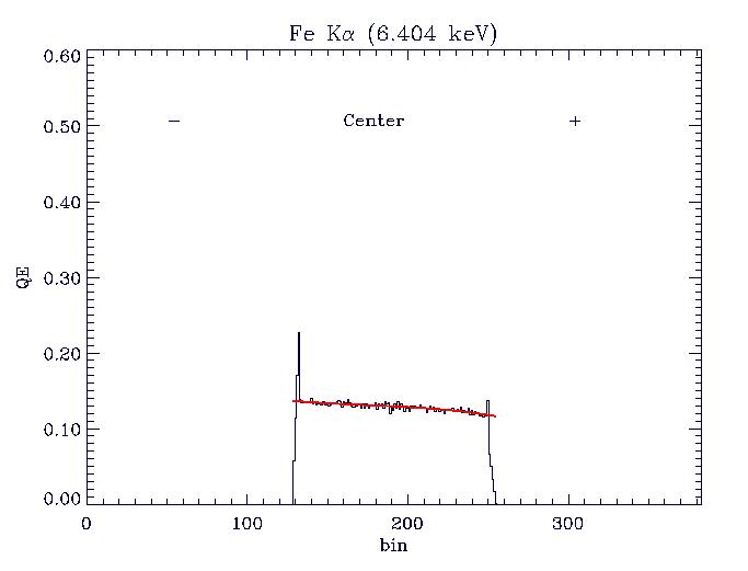
Al K - 1.487 keV	Ti K - 4.511 keV	Fe K - 6.404 keV

NOTE: Only the nominal LETG dispersion strip was extracted from the flatfields because we have detailed source coverage of this region by in-flight calibration sources for confirmation.

Next, an energy grid spanning the full range of interest (0.06 - 12.0 keV) was interpolated/extrapolated from the energies of the data sets. The shapes of the fit polynomial curves were also interpolated/extrapolated to the energy grid to produce an energy-dependence of the QE Uniformity within the nominal extraction region. This narrow QEU strip was then replicated in the cross-dispersion dimension to produce an energy-dependent model of the QEU covering the entire detector, QEU(x,y,E), which is applicable to any pointing of the HRC-S. A more detailed characterization of the cross-dispersion dimension will be pursued as data becomes available. For an example of the function of the QEU, if we take a transection of the data cube at HRC-S nominal aimpoint, we get the QEU line for the nominal LETG dispersion, QEU(0,y,E) [where we assume x=0 is HRC-S nominal aimpoint and y is along the dispersion axis]. This QEU line is shown Figure 4.

Figure 4: HRC-S QEU line for nominal LETG dispersion.

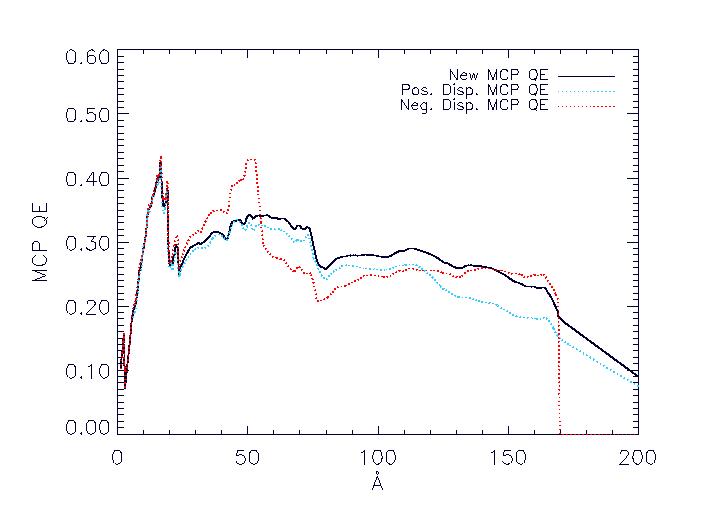
Summary Plot: HRC-S on-axis MCP QE versus LETG dispersion MCP QE
In order to show the effects of the QEU along the HRC-S dispersion axis, in Figure 5 we plot the on-axis MCP QE (black curve) and compare it with the MCP QE for LETG Positive (blue curve) and Negative (red curve) lines of dispersion. Notice not only how different the LETG dispersed QE lines are from on-axis QE, but also how vastly different they are from each other. The difference illustrated in this example is accounted for by the HRC-S QEU line for nominal LETG dispersion, already seen in Figure 4 (above).

Figure 5: HRC-S on-axis MCP QE (black) and LETG dispersion MCP QE,
Positive (blue) and Negative (red) dispersions are plotted separately.

Previous Analyses:
An analysis of the HRC-S results from the ground calibration at the XRCF is also available.

Comments to CxcCal@cfa.harvard.edu

Last modified: 09/25/12

The Chandra X-Ray Center (CXC) is operated for NASA by the Smithsonian Astrophysical Observatory. 60 Garden Street, Cambridge, MA 02138 USA.    Email: cxcweb@head.cfa.harvard.edu Smithsonian Institution, Copyright © 1998-2004. All rights reserved.