ACIS radiator illumination package
Calculate Earth illumination of the ACIS radiator.
The key components are:
- taco.py
- Module which defines the physical geometry and does the raytrace calculations
- acis_rad_illum.py
- Application program using the taco module to calculate illumination over a time range using a supplied orbital ephemeris file. This code generates an output plot and data file and can be used to make gif movies of visibility.
Installation
Untar the package tar file in a working directory:
tar zxvf /proj/sot/ska/export/taco-<version>.tar.gz
cd taco-<version>
acis_rad_illum.py
Calculate Earth illumination of the ACIS radiatiator over a specified interval of time.
Options
-h, --help            show this help message and exit
--tstart=TSTART       Start time
--tstop=TSTOP         Stop time
--ephemfile=EPHEMFILE
                      Orbit ephemeris file containing start and stop times
--out=OUT             Output root name
--sample=SAMPLE       Sample
--ngrid=NGRID         Number of rays to illuminate Earth disk
--nproc=NPROC         Number of processors to use
--verbose             Print verbose output
--movie               Create visibility images for making a movie
The time inputs are tstart and tstop. These can be in any format supported by Chandra.Time.
The orbital ephemeris covering that time range must be supplied in a single file specified by ephemfile. Normally that would be a CXC ORBITEPHEM file, but any file (FITS or ASCII) with the columns Time, X, Y, Z will work.
The output root is given by out. Output files are out.png (illumination vs. time) and out.fits (illumination data). If movie is selected then the visibility images are put in a directory out/.
The illumination calculations will be for one out of each sample values. The default for sample is 2 and the normal time period of CXC ephemeris files is 300 seconds. That implies an output value each 600 seconds.
The number of rays projected toward the Earth is given by ngrid. Rays are only projected toward the “cap” on the surface which would be visible if there were no occultation by the ACIS sun shade. The default is 100 which gives decent resolution over the surface. For making high-resolution movies that could be increased, while for quick calculations a value of 50 might be sufficient.
The number of CPU processors that are used is given by nproc. Default is 4.
The movie option implies creating a visibility image at each time step. To prevent accidentally making a huge number of images the program will stop if an attempt is made to create more than 250 frames.
Examples
The tar file includes an orbital ephemeris file orbitf352123502N001_eph0.fits covering 2009:059 to 2009:128 inclusive.
This is a raytrace code so run it on your fastest multicore machine!
Calculate illumination for a week:
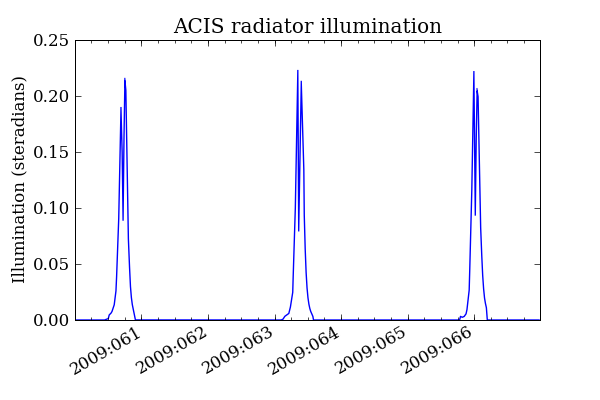
./acis_rad_illum.py --tstart=2009:060:00:00:00 --tstop=2009:067:00:00:00 --out=2009_060_067 --sample=4
gthumb 2009_060_067.png
dmlist 2009_060_067.fits cols
This should result in a plot like

You might get some ominous looking error message like:
Exception exceptions.OSError: (2, 'No such file or directory', '/tmp/tmp_nnyXP.fits')
in <bound method _TemporaryFileWrapper.__del__ of <closed file '<fdopen>',
mode 'rb+' at 0x2c58b70>> ignored
Fear not, this is benign. It is related to the multiprocessing but I haven’t figured out how to get rid of it yet.
Make a movie of a perigee pass:
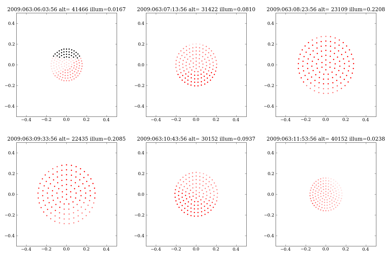
./acis_rad_illum.py --tstart 2009:063:06:00:00 --tstop 2009:063:12:00:00 --out 2009_063_movie --movie
convert -delay 30 2009_063_movie/*.png -loop 0 2009_063_movie.gif
gthumb 2009_063_movie.gif
This should give a movie like below (except this was made with -loop 1 so refresh your browser to see it go):

Note: command line options can use the “=” (equals sign) or not depending on your preference.
taco
Define geometry for ACIS radiator and sunshade and perform raytrace calculation of Earth illumination on the radiator surface.
Functions
- taco.calc_earth_vis(p_chandra_eci, chandra_att, ngrid=100, planes=None, p_radiators=None)
Calculate the relative Earth visibility for the ACIS radiator given the Chandra orbit position p_chandra_eci and attitude chandra_att.
The relative visibility is normalized so that 1.0 represents the entire radiator having visibility toward the surface point and being exactly normal toward the surface.
Total illumination gives the effective solid angle (steradians) of the visible Earth from the radiator perspective. It is averaged over the different points on the radiator.
Parameters: - p_chandra_eci – Chandra orbital position [x, y, z] (meters)
- chandra_att – Chandra attitude [ra, dec, roll] (deg)
- ngrid – number of points on visible Earth to raytrace
- planes – list of Plane objects defining structure
- p_radiators – points on radiator surface
Returns: relative visibility, total illumination, projected rays
- taco.make_radiator()
- Specify points on the ACIS radiator surface.
- taco.make_taco()
- Define geometry for ACIS radiator sun-shade (aka the space taco).
- taco.plane_line_intersect(p, l)
Determine if the line l intersects the plane p.
Return type: boolean
- taco.sphere_grid(ngrid, open_angle)
Calculate approximately uniform spherical grid of rays containing ngrid points and extending over the opening angle open_angle (radians).
Returns: numpy array of unit length rays, grid area (steradians)
- taco.quat_x_v2(v2)
- Generate quaternion that rotates X-axis into v2 by the shortest path