

The Iris GUI uses the STILTS API for its plotting backend. The tabular and plot displays of SED data are heavily based on STIL, the library both TOPCAT and STILTS use. This thread presents the various options available for interacting with and customizing the SED data display in the Iris Visualizer.
Last Update: Feb 22 2017 - Updated images and text for Iris 3.0.
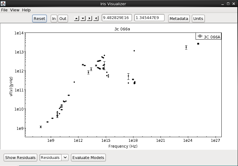
When SED data is read into Iris, it displays in the Iris Visualizer, where you can interact with the data plot in various ways. You can open the Iris Visualizer from the desktop icon “Iris Visualizer.” The terms Iris Visualizer and SED Viewer are used interchangeably throughout the documentation. The options available for customizing the data display are described in this thread.
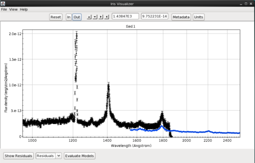
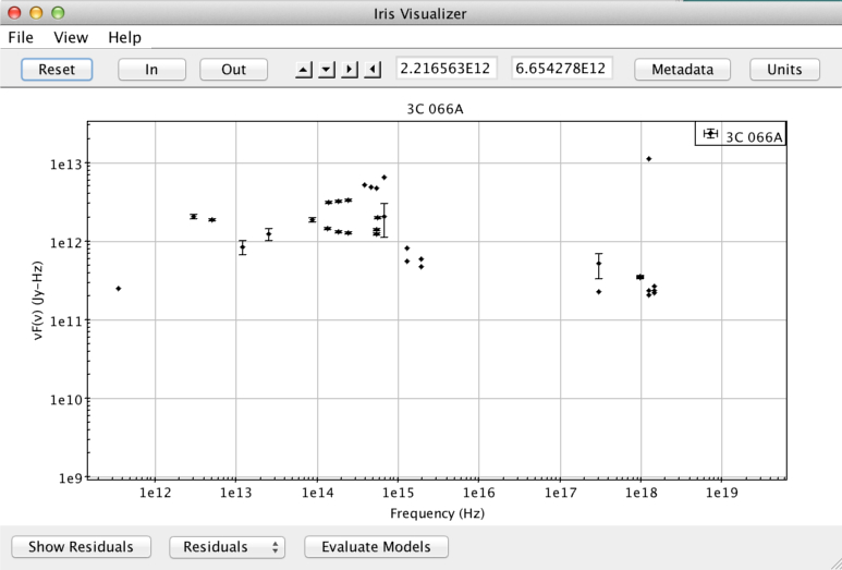
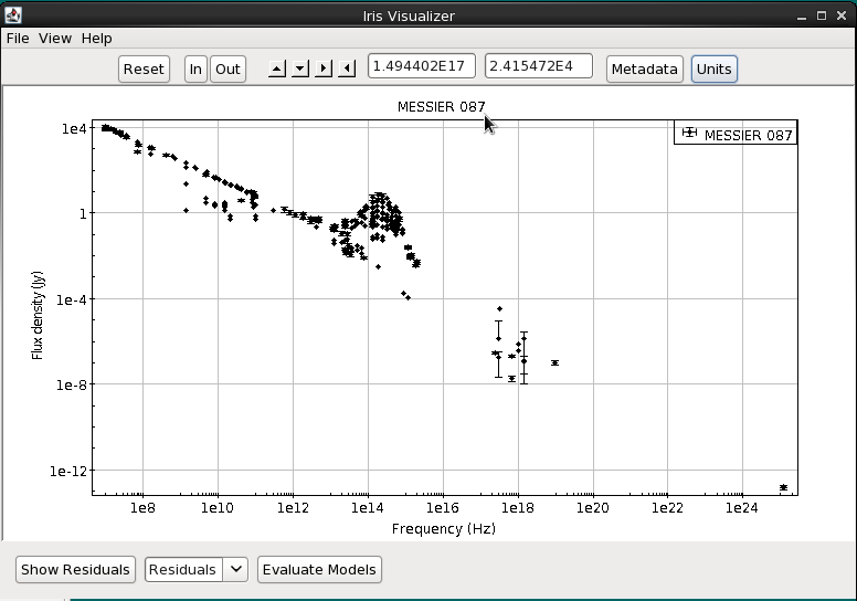
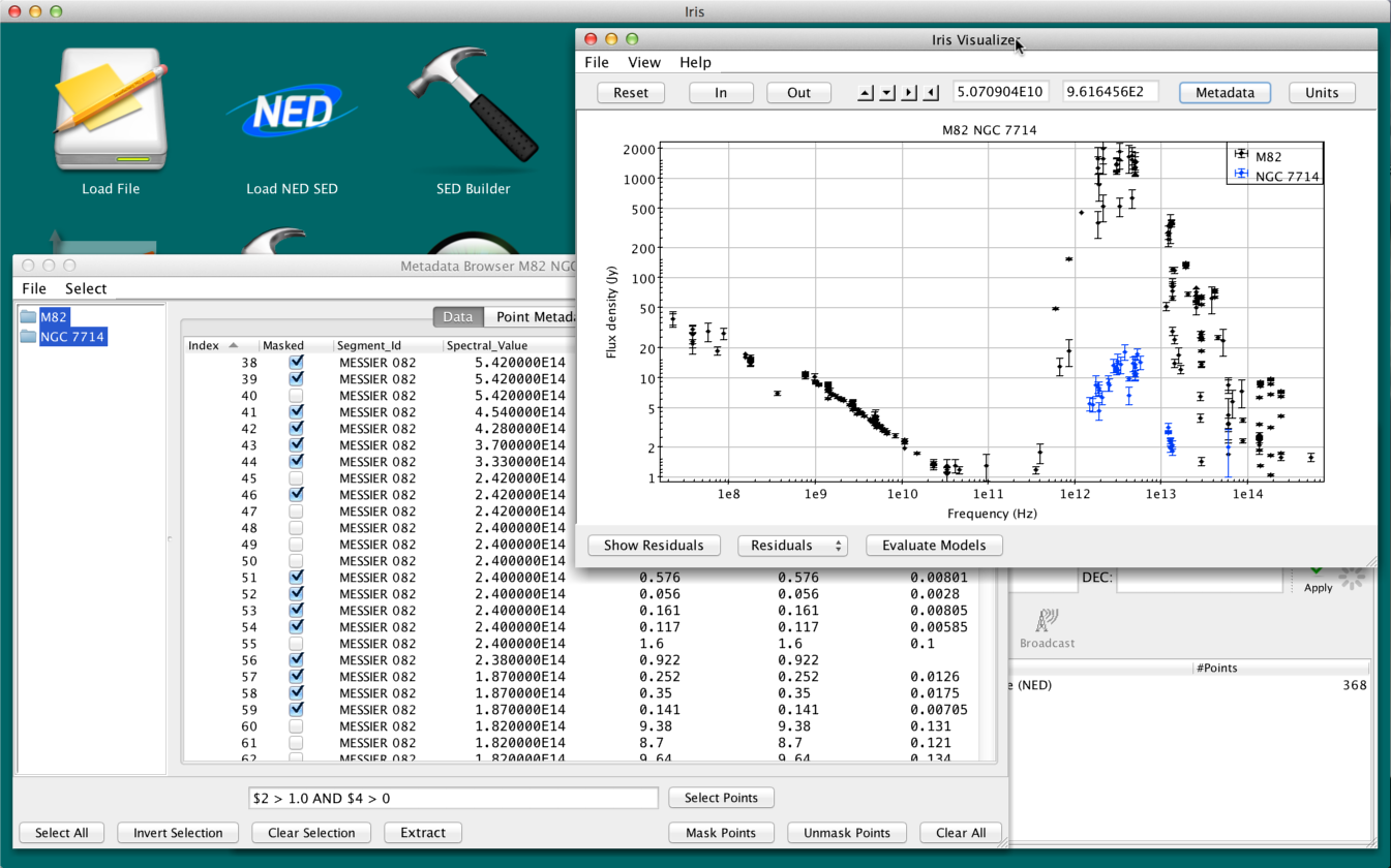
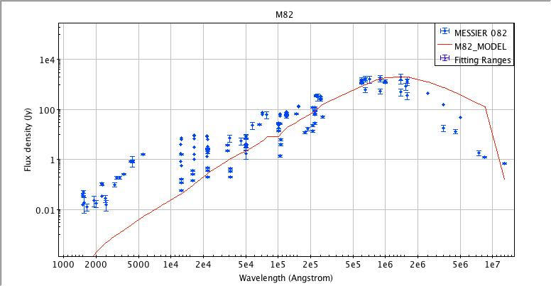
When multiple segments and/or photometric points have been read into the Iris session and co-plotted in the main display, it is important to note that the spectral data are not combined, co-added, or spliced in memory in any way; the raw data from the multiple input spectrograms/points is completely preserved in the resulting combination. This means that two separate SED data segments loaded into Iris for a particular source - e.g., observed with two different observatories and spanning separate (or overlapping) spectral ranges - may be offset from one another, as Iris does not automatically scale, trim, and join the separate segments to form a seamless SED for the source. This is illustrated in the image below.
The set of widgets in the Visualizer toolbar are available for adjusting the view and orientation of the SED segment(s) within the main display.
There are a few methods of zooming and out of the view port:
![[Iris screenshot image]](./imgs/zoom_buttons.png) Zoom out/in by 33% from the center of the viewport by clicking the “In” and “Out” buttons at the top of the Visualizer.
Zoom out/in by 33% from the center of the viewport by clicking the “In” and “Out” buttons at the top of the Visualizer.There are two methods for panning around the view port:
![[Iris screenshot image]](./imgs/left_right_buttons.png) Use the four (4) arrow buttons at the top of the plot window to pan the view port up, down, left, and right.
Use the four (4) arrow buttons at the top of the plot window to pan the view port up, down, left, and right.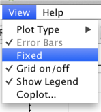
The user may choose to automatically scale the coordinates view port to fully encompass the data each time the plot is refreshed; or, fix the coordinates view port so that all subsequent plot refreshes that result from a data change will take place on a fixed coordinates view port. To choose the behavior, toggle “View –> Fixed” preference.
By default, if any SED changes occur (adding/removing a SED segment, switching SEDs, etc.), the plot ranges will automatically be reset to show every data point in the SED. By fixing the plot, any SED events that happen outside of the Visualizer will not affect the view port plot ranges. The user can still pan, zoom in/out, and reset the plot ranges manually; the plot view will remain unaffected only by SED changes.
![[Iris screenshot image]](./imgs/reset_button.png) The “Reset” button is available within the Iris main display for resetting the data plot so that all edges. |
The “Reset” button is available within the Iris main display for resetting the data plot so that all edges. |
 The preferred units for the data display, e.g., “ergs/cm2/s/angstrom” versus “angstrom”, may be set using either the “Units” button in the upper-right corner of the main display. This also updates the units shown in the Metadata Browser’s “Data” tab.
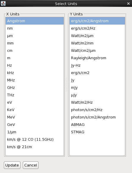
The “Units” button allows you to choose the spectral and flux/flux density units to display an SED in. A dialog box populated with all available physical units will pop up: the left column is for the spectral (X) axis, and the right column holds the flux/flux density axis. Selecting the desired units and clicking the “Update” button adjusts the data display to the desired preference.
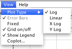
The X and Y axes can be plotted in linear or logarithmic scales. The user controls the scaling by clicking “View –> Plot Type –>” on the menu bar, then choosing the scaling.
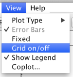
Selecting the “Grid” option in the main display overlays a coordinate grid onto the main plot.
| [Back to top] |
Be default, a plot legend is shown in the top-right corner of the plot display. The legend can be hidden/shown by checking the preference “View –> ”Show Legend" off and on.
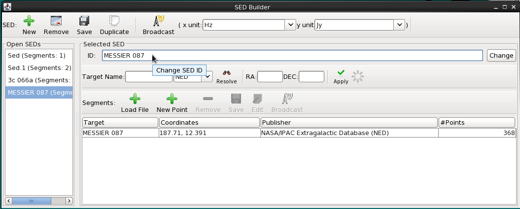
By default, the SED Viewer window displays either “Sed” or “Iris Visualizer” for any file loaded into Iris. This name can be changed in the SED Builder window. Type the desired name in the bar next to “ID:” under “Selected SED” then click “Change.” From now on, the SED Viewer window will display the new name on the top bar and on the plot.
| [Back to top] |
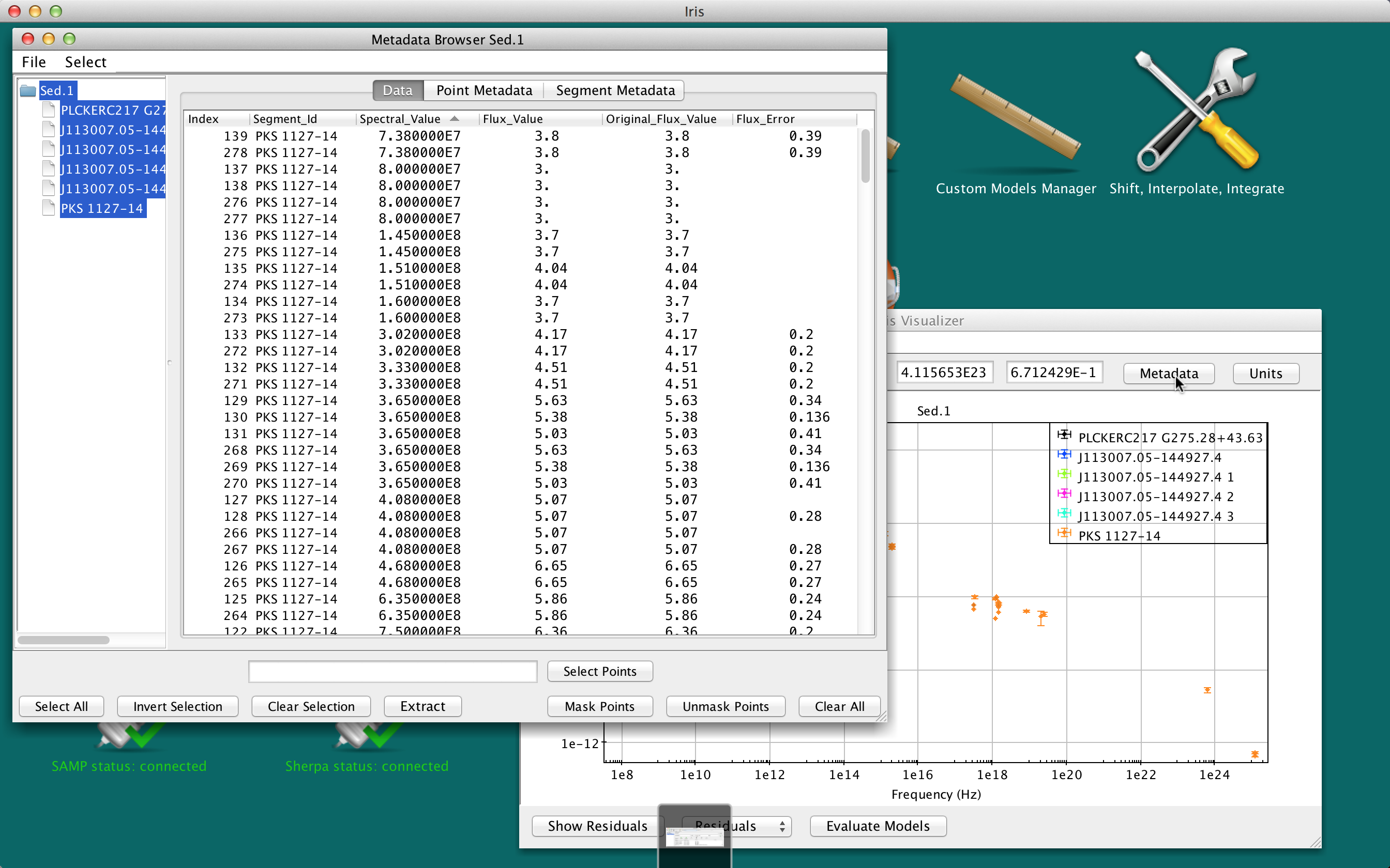
Clicking the “Metadata” button in the upper-right corner of the Iris display opens a window with tabs containing different levels of data and metadata in the SED.
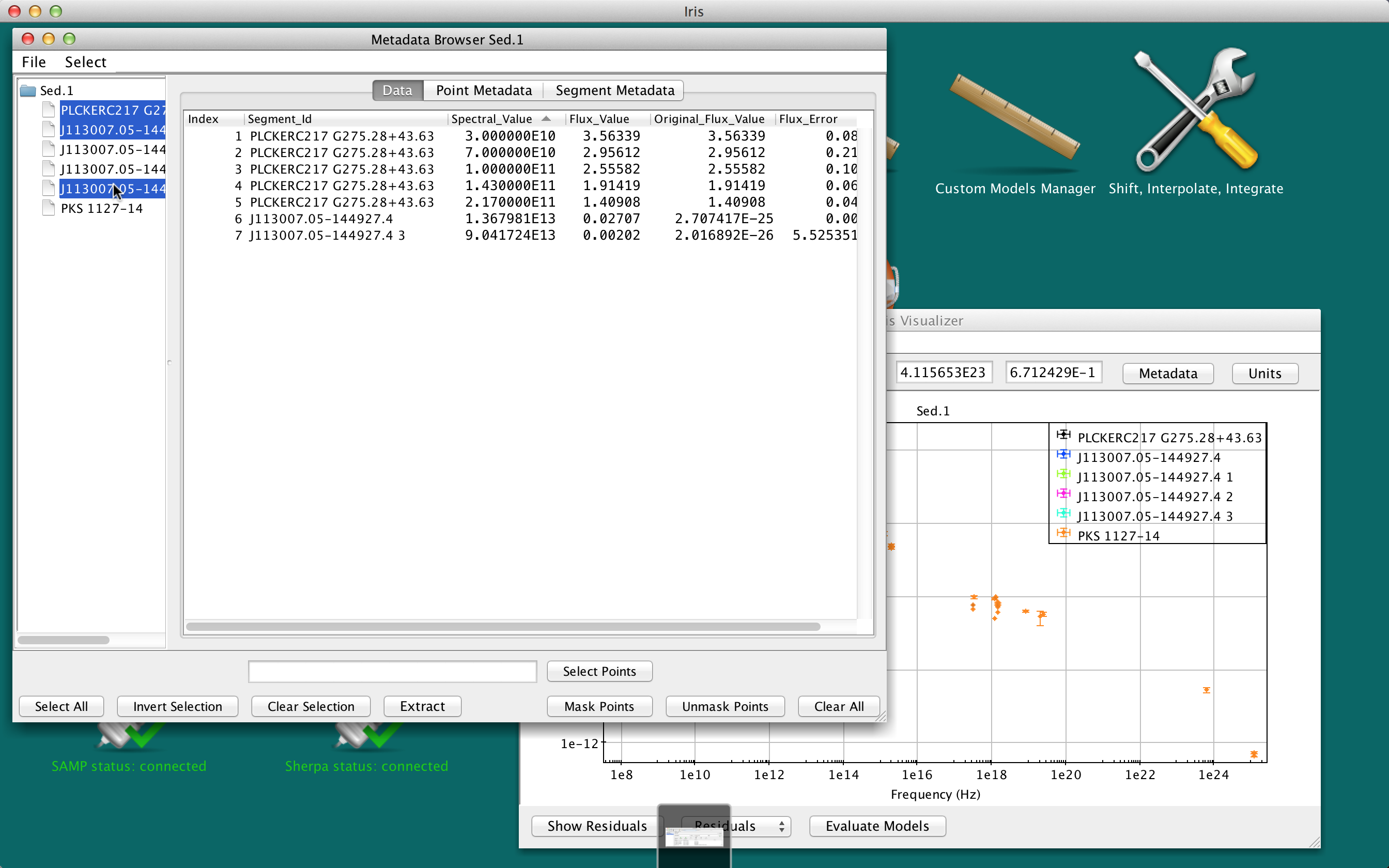
The metadata tables may be sorted by clicking the header of the column by which you would like to sort - once for ascending order, twice for descending order - and rearranged by clicking and dragging columns left or right.
Users can view the metadata of an arbitrary selection of SED Segments from the left column. Hold down Shift and click on the Segments you wish to display in the Metadata Browser tabs. The rows in the Data and Point Metadata tabs will update to the highlighted SED segments.
These sections use VOTable pks1127-14.vot for demonstrating the Metadata Browser. Refer to Loading SED Data into Iris if you need instructions on loading files from disk.
The X and Y coordinate values of each SED data point in the Iris display are contained in the “Spectral Axis” and “Flux Axis” columns of the Data tab, and reflect the values that are currently plotted in the Iris display; when the plot units are changed, the Data tab updates accordingly.
| [Back to top] |
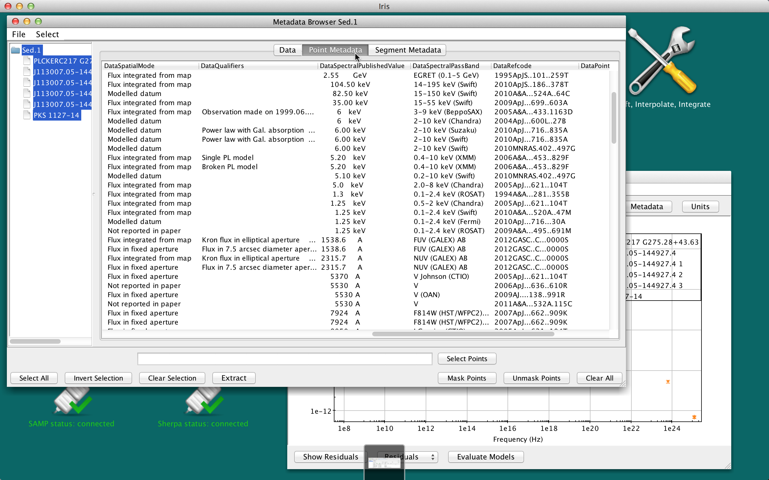
When available, the Metadata tab includes many useful pieces of information about the data points currently displayed. When a SED is imported from NED, as in the example considered in this thread, the metadata includes such things as the bibliographic reference code for each data point, the spectral range covered by instrument used to obtain data point, data point uncertainty and flux values as they are published, data point significance values, among other properties. The full list of metadata information available for each data point will depend on the specific data sources.
| [Back to top] |
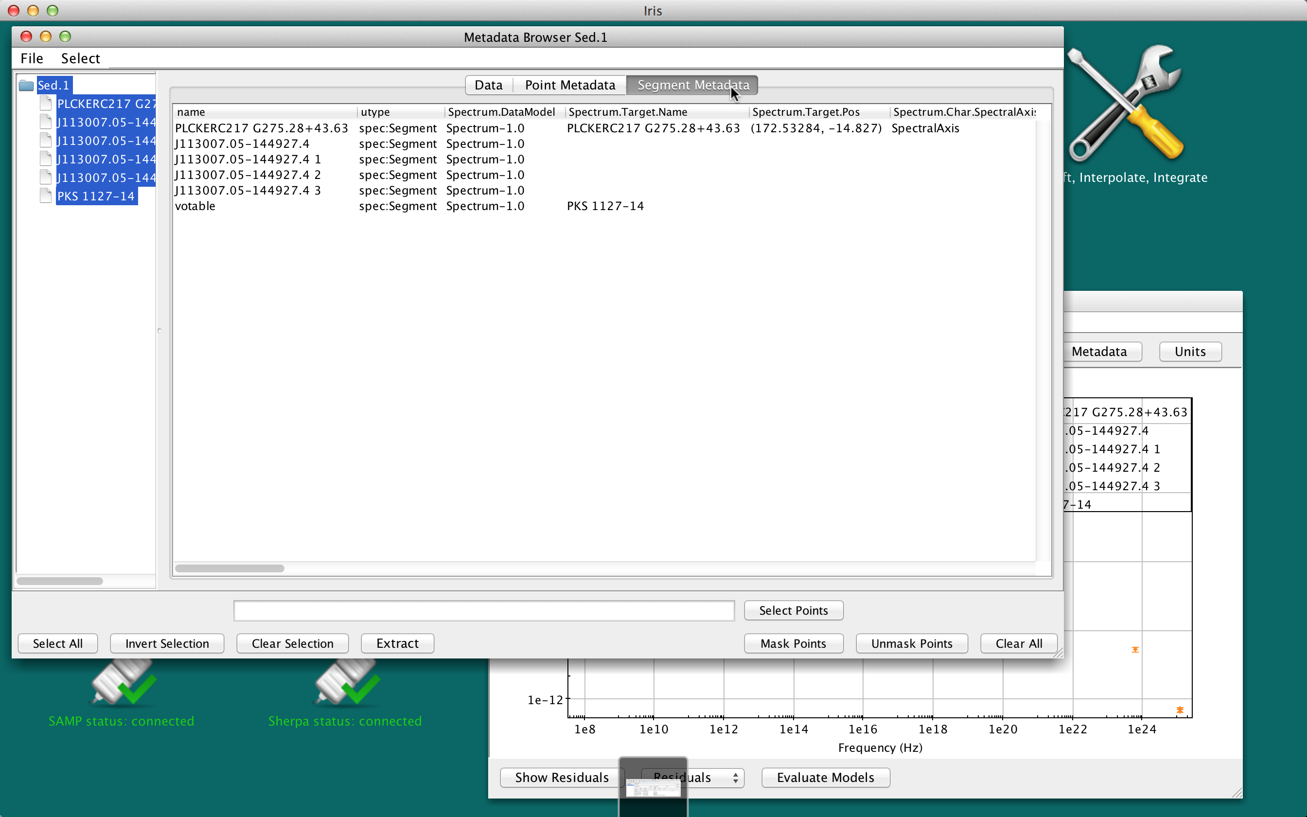
Metadata that is common to all data points in a SED segment is displayed under this tab, in a similar table as the one that appears under the Point Metadata tab.
| [Back to top] |
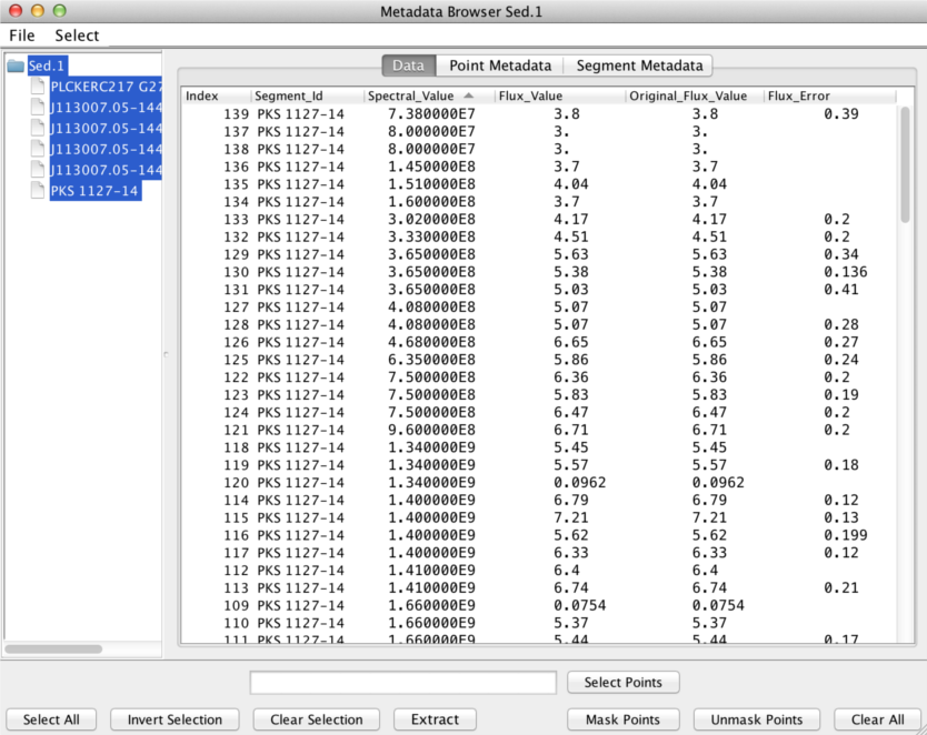
Users can filter and mask SED data using various tools in the Metadata Browser. These capabilities can be accessed from the toolbar under “Select –> ”, or through the convenience buttons at the bottom of the Browser window.
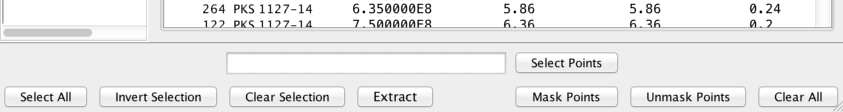
Here is a quick reference list to the Metadata window’s filtering tool buttons:
 - select all the points in the table
 - invert the selection of points
 - clear all point selections
 - create a new SED out of the selected points
 - mask the selected points. These points will be hidden from the plot and will not be included in any fits
 - unmask the selected points.
 - clear all masks
 - select the rows for which the given filter expression returns True.
The subsections below describe in more detail how users may view, filter, and extract new datasets from their SEDs.
Data points can be masked from the Iris plot display and fitting sessions with a number of methods.
The most basic works by simply selecting the rows corresponding to these points in any one of the Point Metadata or Data tabs of the Metadata window, and then clicking “Mask Points” at the bottom of that window. You can select the points by clicking the desired rows while pressing the Ctrl/Command key. In the display, the selected points will be removed.
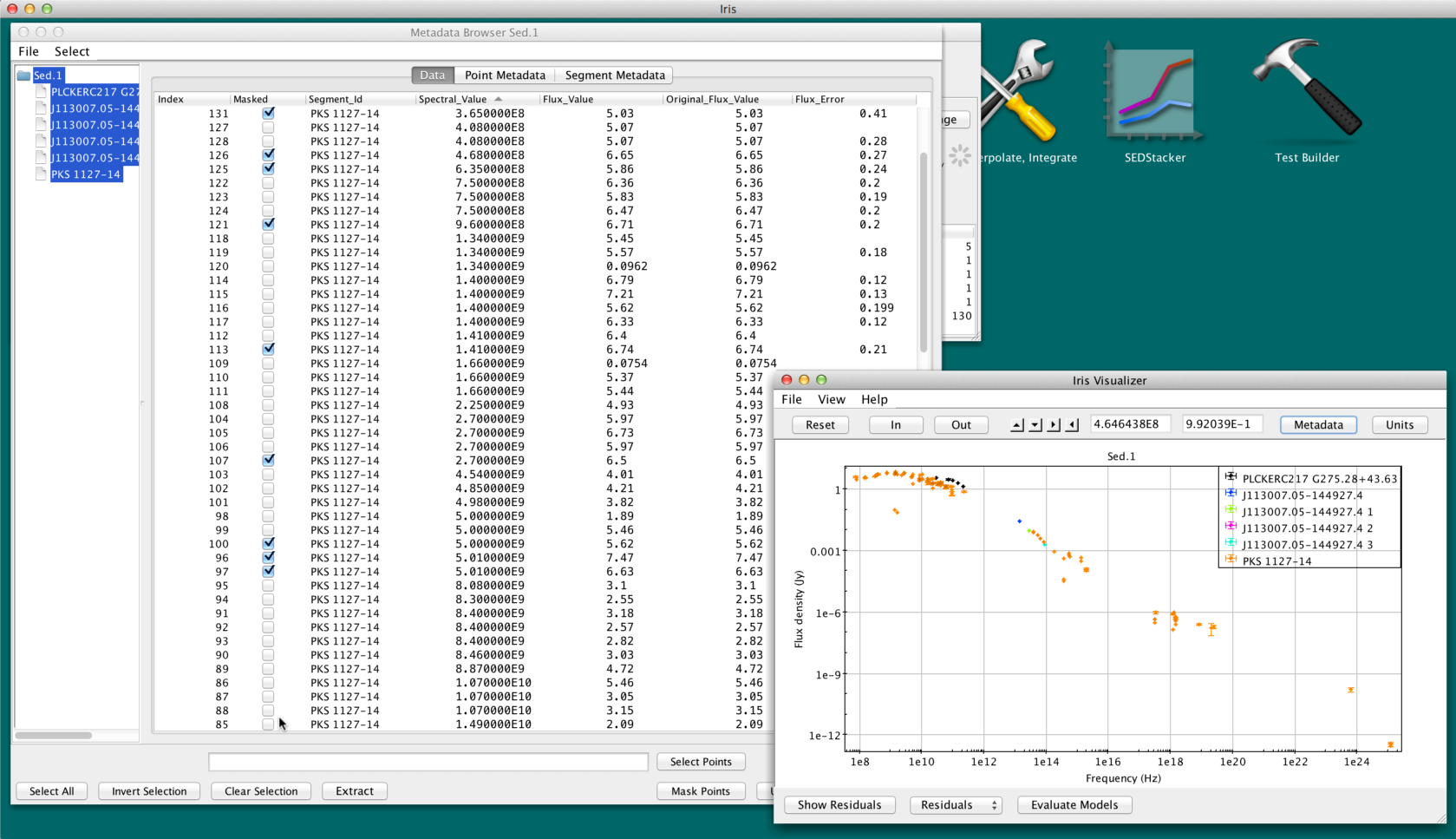
In the Metadata Browser, masked points are denoted by a checkmark in the “Masked” column. The “Masked” column is only present when at least one point is masked. Note that this checkbox column is not clickable; to mask/unmask points, select the rows you wish to edit, then click or .
The Data and Point Metadata tables can be hierarchically sorted by clicking on specific column headers. Clicking once sorts the rows in ascending order of that column; the next click sorts it in descending order . Using that mechanism, rows can be re-ordered together according to relatively complex selection criteria against column content. This facilitates the lumping together of the desired rows, that can in turn be selected and operated upon with the tools described in the preceding paragraph.
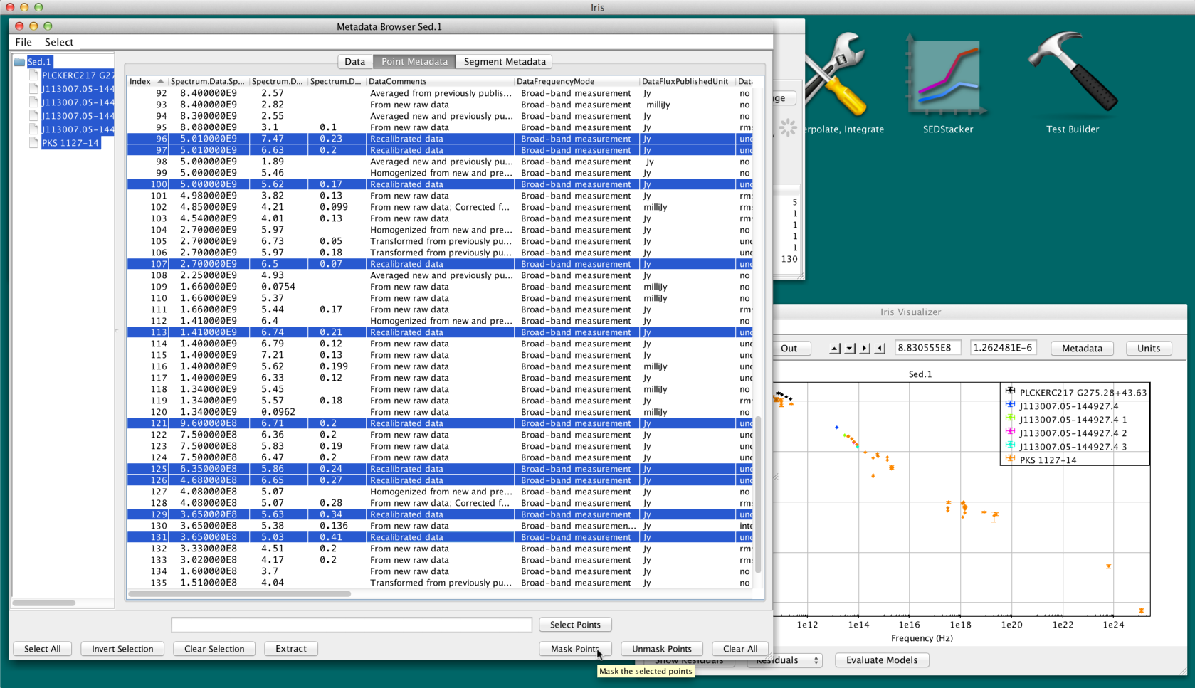
For example, we can click on the “DataComments” column and easily mask data points with values “Recalibrated Data” by holding down the Shift key and clicking the top and bottom of the “Recalibrated Data” block in the table (see figure below).
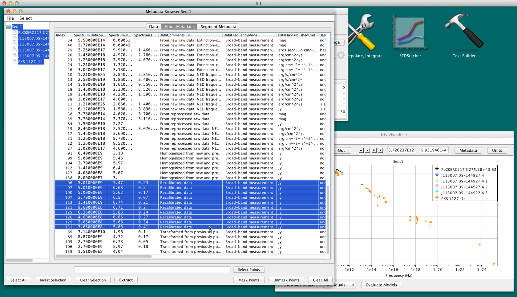
Note that columns can be re-positioned at will by dragging their headers horizontally.
Also note that string-valued columns are treated in lexical order. Integer and floating-point-valued columns are treated in numerical order.
| [Back to top] |
Data point selection can also be performed based on the plot itself, instead of the table. One way to do that is by clicking on a specific data point on the display. The corresponding row in both the Point Metadata and Data tables will be selected. This selection is non-destructive, meaning that by successively clicking on points on the display, one can add the rows corresponding to each one, to the set of selected rows.
| [Back to top] |
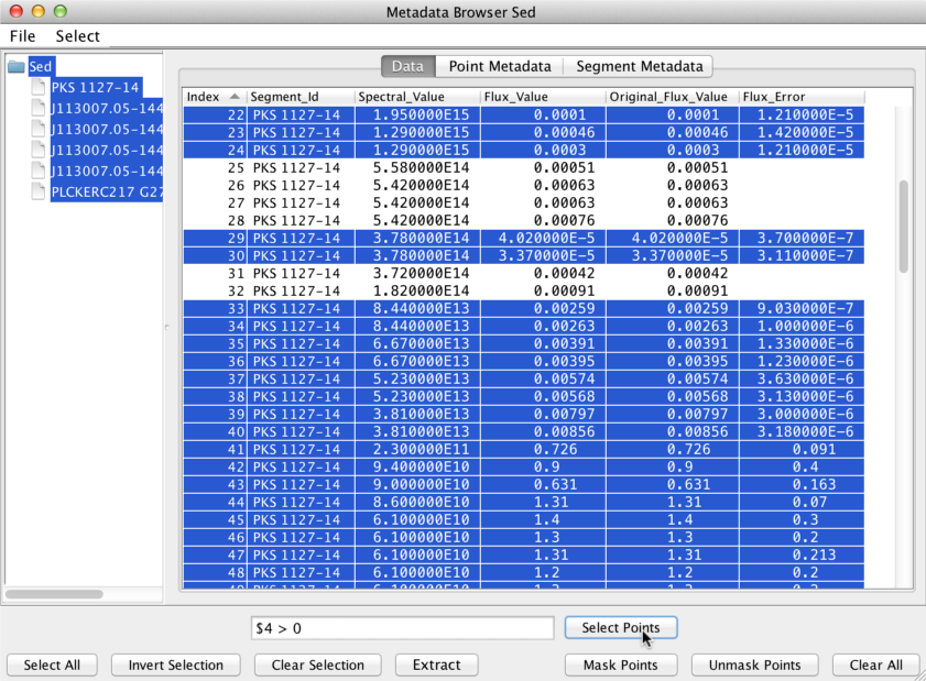
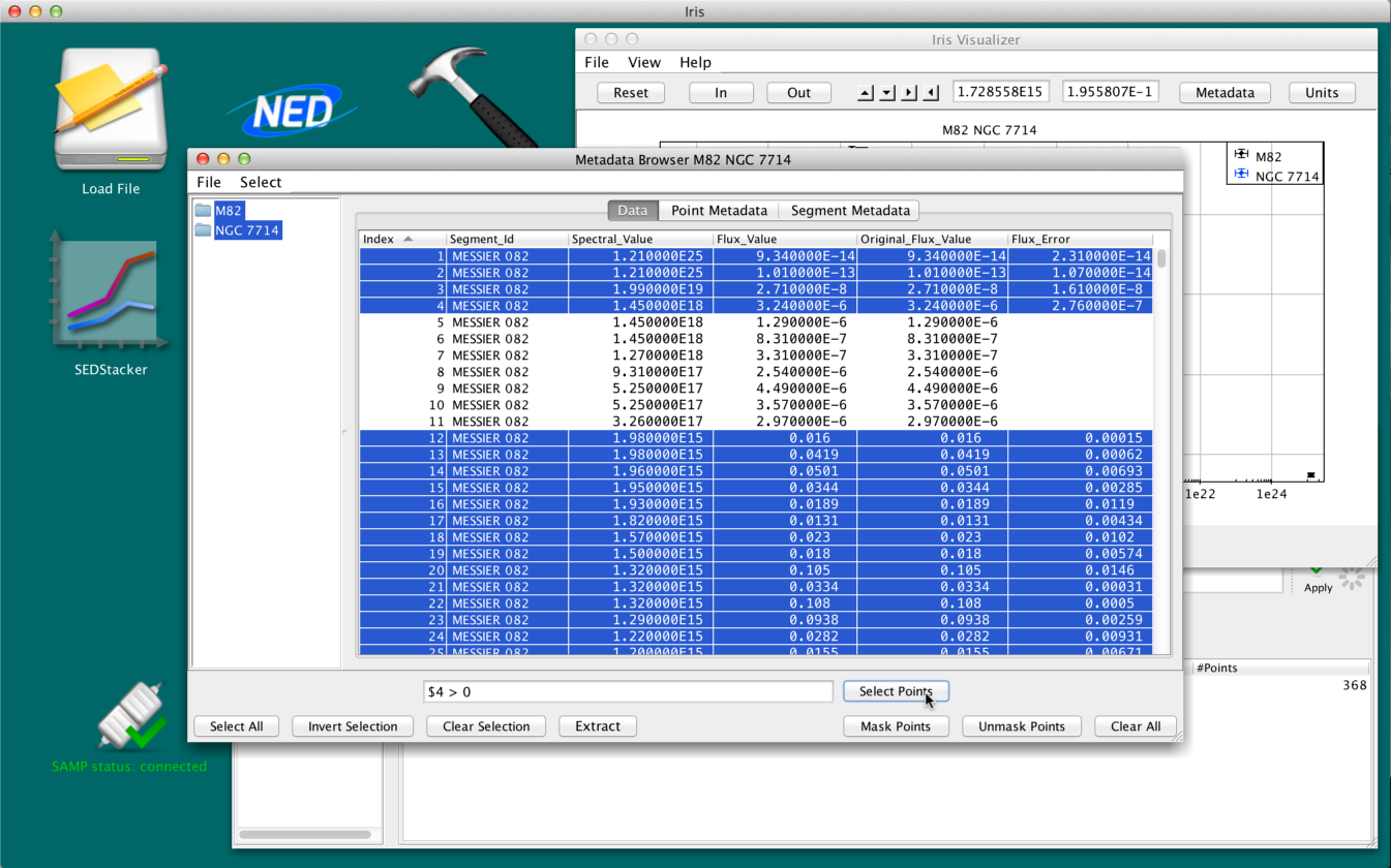
In order to enable even more complex selection criteria though, table rows can be selected based on the result of an arbitrary Boolean expression computed on selected column contents. This expression is entered in the ‘Filter Expression’ text field, and by hitting Return, or clicking on the ‘Select points’ button, the expression is computed for every row in the table, and the row is selected if the Boolean result is True.
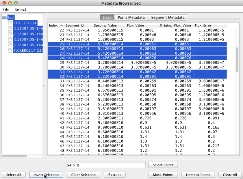
In the expression, columns are referred by their ordering, where the first column is 0. Columns are specified by a “$” followed by the column number. For example, given the table below, one may select the points which have an associated uncertainty with
$4 > 0
then they can mask the points without associated errors by clicking “Invert Selection”.
Columns may be arbitrarily combined in an expression; what is required are boolean comparisons with at least one column on the left- or right-hand side. Comparisons may be combined with the logical operators AND, OR, and NOT. Expressions are evaluated following the basic order of operations. Iris uses javaluator under the hood as to evaluate numeric expressions. All mathematical operators (*, /, +, -,^,log(),log10()) allowed in javaluator may be used in the filter expression.
| Comparison Operators | Logical Operators | ||
|---|---|---|---|
| == | equal to | AND | “and”; intersection of sets |
| != | not equal to | OR | “or”; union of sets |
| > | greater than | NOT | “and not”; subtraction of sets |
| >= | greater than or equal to | ||
| < | less than | ||
| <= | less than or equal to | ||
s
| Logical Operators | |
|---|---|
| AND | “and”; intersection of sets |
| OR | “or”; union of sets |
| NOT | “and not”; subtraction of sets |
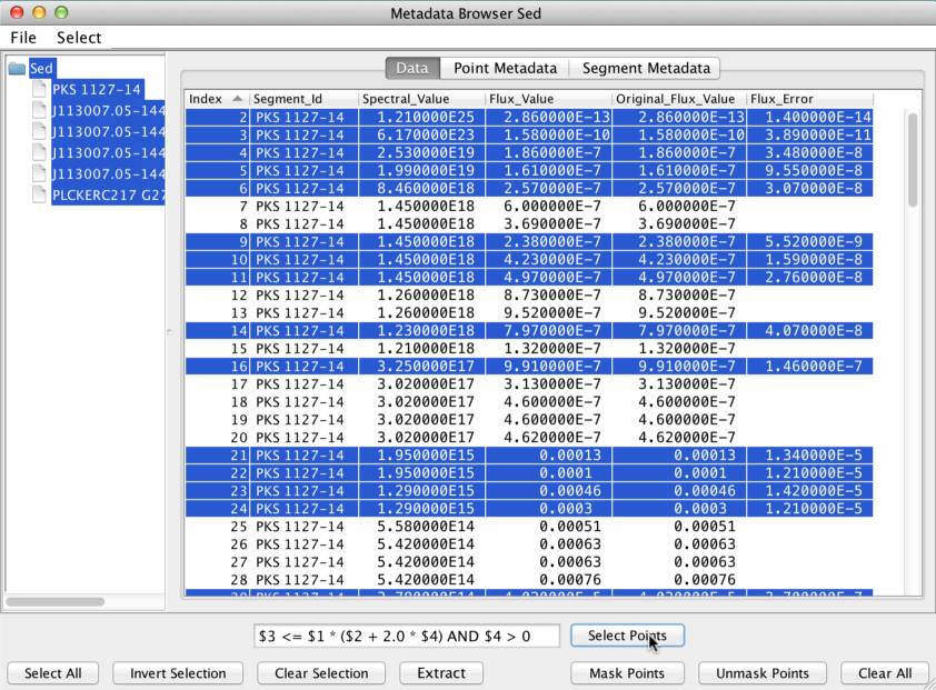
Here is an example of a more complex filter expression:
$3 <= $1 * ($2 + 2.0 * $4) AND $4 > 0
This means “select points where the values in column 3 are less than or equal to the values of (column 2 plus 2 times column 4), all times column 1. Out of these selected points, only pick those whose values in column 4 are greater than 0”.
Caveat: Only numeric columns may be filtered in Iris 3.0.
WARNING: Currently columns may only be specified by their column order. If a user applies a mask to come data points, the new column will push the columns over by 1, so that one must add 1 to their column specifiers in the filter expression. The same applies for a user re-ordering the columns; if the
For example, if the column expression is
$2 > 1.5 * $3
and the user moves the third column to the place of the second column, $2 refers to the current 2nd column, which was previously column 3.
(See more examples of using the Boolean filter in Co-plotting Separate SEDs)
| [Back to top] |
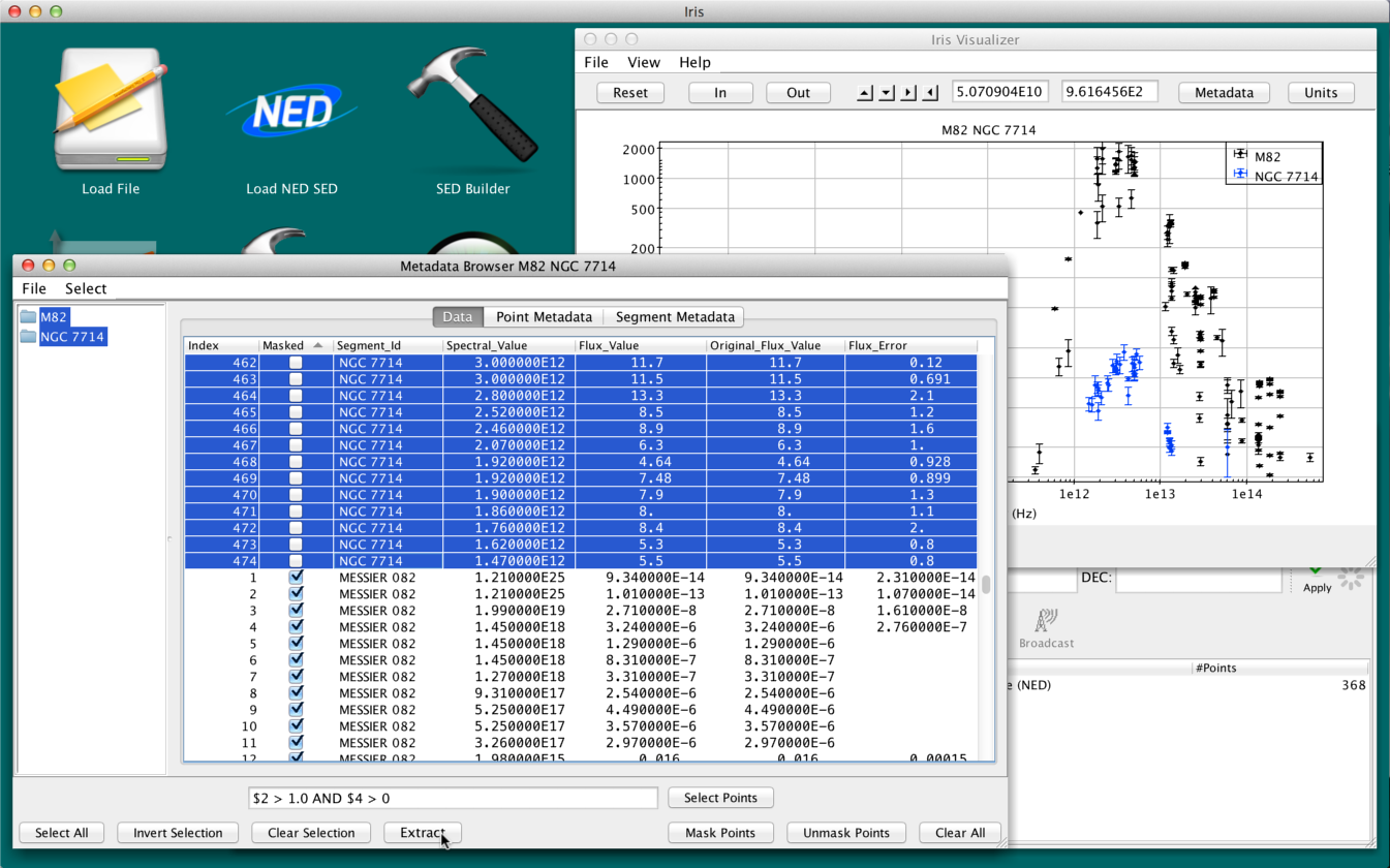
The “Extract” function in the Metadata window allows you to go one step further than simply masking unwanted data points; it allows you to extract a whole new SED consisting of only the selected data points.
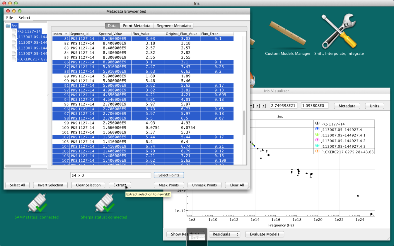
Making the desired row selections in the Metadata window and then clicking “Extract” will open a new SED in the SED Builder window named “FilterSED” - an ID which you can change - which will display in the SED Viewer.
| [Back to top] |
One can simultaneously plot two or more separate SEDs using the Co-plot function in the SED Viewer. In this example, we will co-plot two out of the three separate SEDs imported from NED: M82, M87 and NGC7714.
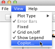
Click the “View” button on the Viewer toolbar (upper-left corner) and select “Coplot…” A menu with the list of all SEDs available for co-plotting will pop up.

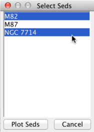
To co-plot, hold-down the Control key (Command key on Mac systems) and click on the SED names you wish to view, and then click the “Plot Seds” button on the menu (to select all SEDs, click on the first SED, hold-down the Shift key, click on the last SED, and hit “Plot Seds”). Here, we’ve selected M82 and NGC7714.
The Visualizer updates with all SEDs selected for co-plotting. Each SED is plotted with a different color, and the color-coding and the names of the SEDs co-plotted are shown in the legend (which can be hidden by unchecking “View –> Show Legend” in the menu bar). Note that the axis units may change after co-plotting; use the “Units” button in the upper-right corner of the SED Viewer if you wish to change the axes units in co-plot mode.
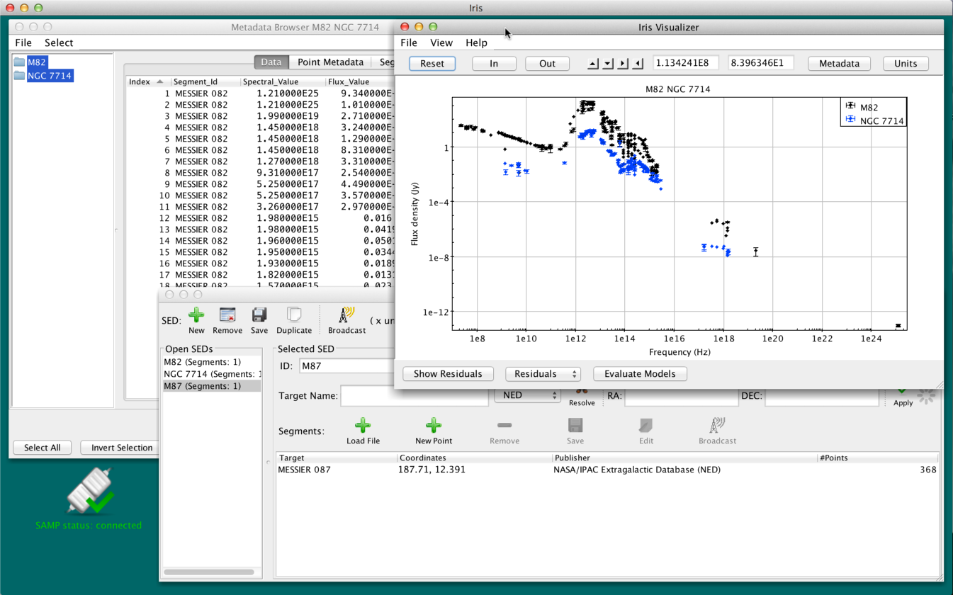
In co-plot mode, you can still access the metadata of each photometric point by clicking on it, and the Metadata Browser (that can be accessed by clicking on the “Metadata” button in the SED Viewer window) can be used to explore the distribution of data and metadata for all photometric points in the plotted SEDs.
In this example, we use the same NED SEDs “M82” and “NGC7714” from above.
In co-plot mode, the Metadata Browser orders the rows by SED first, then by spectral value. This is true for both the Data and Point Metadata tabs. The same filtering, masking, and selection capabilities are available in co-plot mode.
To restore the original row ordering of the co-plotted table, click on the “Index” column in either tab.
Let’s say we’re interested in points with published uncertainties and with flux values larger than 1.0 Jy. We can mask out the other points from the plot and the Fitting Tool. Click on the “Data” tab and type $2 > 1.0 AND $4 > 0 into the Filter Expression field, where $2 is the Flux_Value column, in Jy, and $4 is Flux_Error. We then click “Select Points” –> “Invert Selection” –> “Mask Points”.
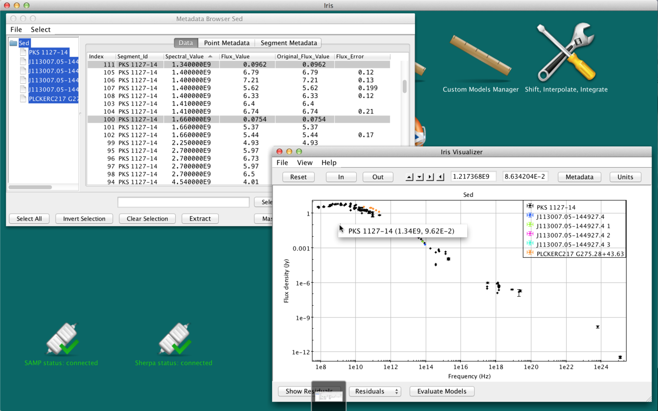
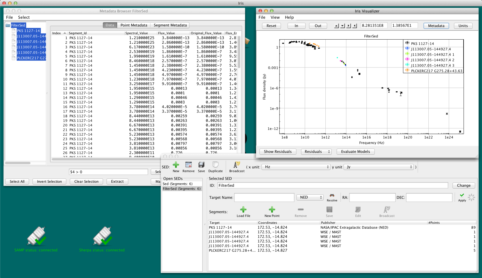
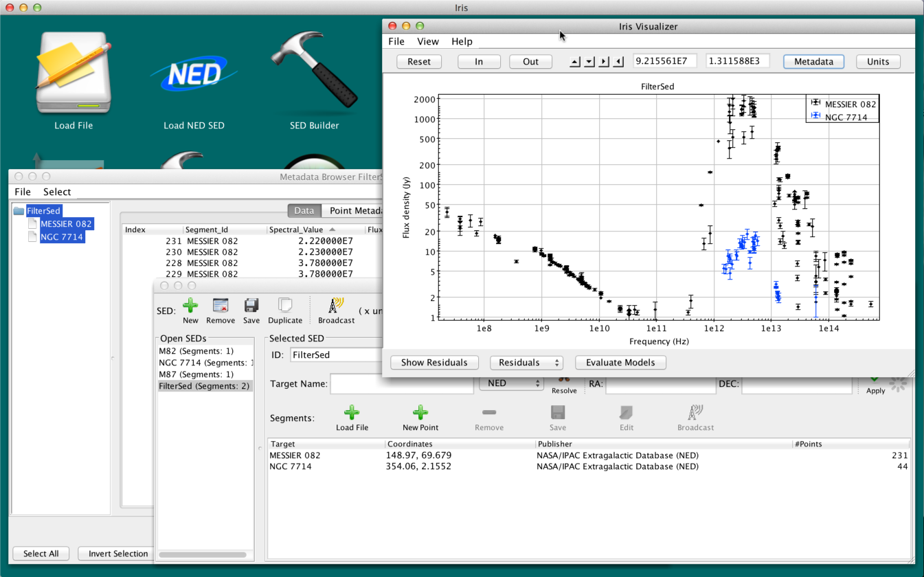
One can “Extract” the desired points to a new SED. If you masked the points in the example above, you can either
or
Either method will produce new SED called “FilterSed.” This SED is displayed in the Viewer, and is available for saving, appending and analyzing from the SED Builder window. The final SED is displayed in the figure below.
| [Back to top] |
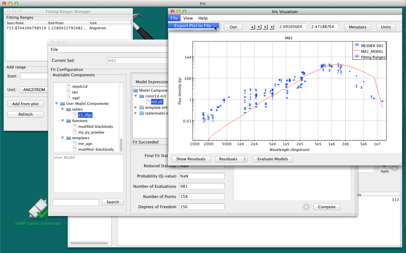
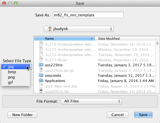
The SED data currently displayed in Iris may be printed to a hardcopy image in either JPG (.jpg), PNG (.png), GIF (.gif) or BITMAP (.bmp) format, by selecting “File –> Export plot to image file”, and making the desired image format selection. The image will scale to the size and shape of the plot in the Iris Visualizer.
| [Back to top] |
Iris is able to communicate with other SAMP-enabled applications, such as Topcat and Aladin. So long as the SAMP status in the lower left-hand corner of the Iris desktop says “connected”, we can transmit tabular data back-and-forth between Iris and other SAMP-enabled Virtual Observatory programs.
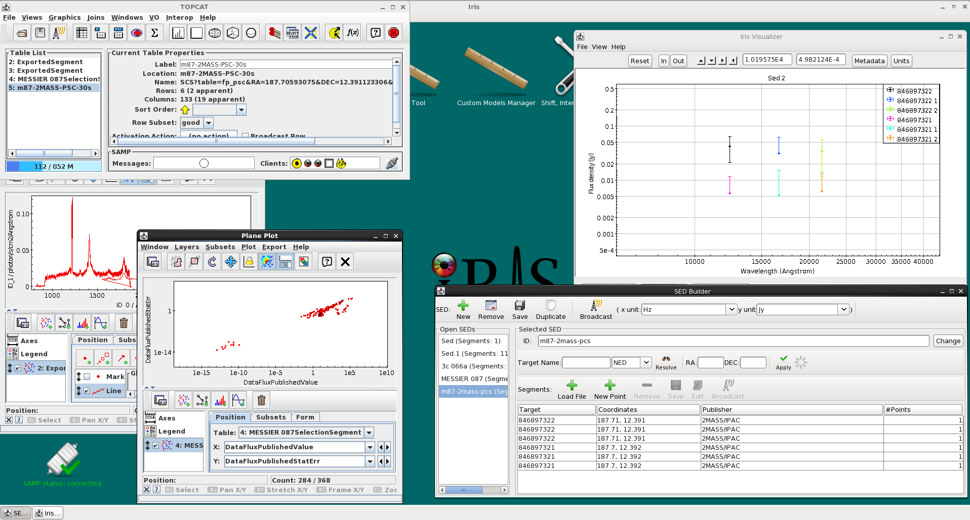
Data is transferred between different applications through the “Broadcast” button. Iris can broadcast data from the SED Builder, which allows us to send the metadata for SED segments and aggregate SEDs, and from the Metadata Browser, from which we can select specific data points to send using the same methods outlined above in this thread (selecting by column, Boolean filter, selecting from plot, etc.). The button is located at the top of the SED Builder window, symbolized as a radio tower, and in the bottom right-hand corner of the Metadata Browser window.
Say we want to explore the 3C 066A data with published uncertainties in a program more suitable for tabular data manipulation, for example Topcat. We first mask data without uncertainties using the Boolean filter in the Metadata Browser. If Topcat is open (see TOPCAT documentation), you should be able to send the table containing all metadata of the selected subset of points to Topcat by simply clicking on the “Broadcast” button in the Single Point metadata browser tab (just make sure that Iris is registered to the SAMP hub by checking whether Iris icon appears in the lower-right margin of the main Topcat window). At this point, a table of the metadata of the selected points will appear in the Topcat file list window, where users will be able to produce scatterplots, histograms, and harness all of the powerful data manipulation and data discovery features available in Topcat.
| [Back to top] |
| Date | Changes |
|---|---|
| 08 Aug 2011 | updated for Iris Beta 2.5 |
| 26 Sep 2011 | updated for Iris 1.0 |
| 12 Jun 2012 | updated for Iris 1.1 |
| 27 Nov 2012 | updated for Iris 1.2 |
| 05 Aug 2013 | Updated for Iris 2.0. Added co-plot capability, interoperability with SAMP-enabled applications, and saving plot images discussions. Updated screenshots and fixed table of contents. |
| 02 Dec 2013 | Updated for Iris 2.0.1 |
| 07 May 2015 | Updated for Iris 2.1 beta. |
| Jan 03 2017 | Updated text for Iris 3.0. |
| Feb 22 2017 | Updated images for Iris 3.0. |
| [Back to top] |