Mica Archive
The Archive components of the mica suite provide tools to:
- retrieve telemetry and processed products from the CXCDS archive
- store these products in a Ska file archive for speed and convenience
- quickly retrieve these products
Mica provides interfaces to these products:
ACA dark current
The mica.archive.aca_dark package provides modules related to the ACA dark current:
Dark current calibrations
The mica.archive.aca_dark.dark_cal module provides functions for retrieving data for the ACA full-frame dark current calibrations which occur about four times per year (see the ACA dark calibrations TWiki page).
The functions available are documented in the mica.archive.aca_dark section, but the most useful are:
- dark_temp_scale(): get the temperature scaling correction
- get_dark_cal_dirs(): get an ordered dict of dark cal identifer and directory
- get_dark_cal_image(): get a single dark cal image
- get_dark_cal_props(): get properties (e.g. date, temperature) of a dark cal
- get_dark_cal_props_table(): get properties of dark cals over a time range as a table
As an example, let’s plot the raw and corrected warm pixel fraction over the mission. The correction in this case is done to a reference temperature of -15 C:
from mica.archive.aca_dark import dark_cal
from Ska.Matplotlib import plot_cxctime
from Chandra.Time import DateTime

dark_cals = dark_cal.get_dark_cal_dirs()
times = []
n100 = []
n100_m15 = []
npix = 1024. * 1024.

for dark_id in dark_cals:
    print('Reading {}'.format(dark_id))
    props = dark_cal.get_dark_cal_props(dark_id, include_image=True)
    scale = dark_cal.dark_temp_scale(props['ccd_temp'], -15.0)
    image = props['image']
    times.append(props['date'])
    n100.append(np.count_nonzero(image > 100.0) / npix)
    n100_m15.append(np.count_nonzero(image * scale > 100.0) / npix)

times = DateTime(times).secs
figure(figsize=(6, 4))
plot_cxctime(times, n100, 'o-', color='red')
plot_cxctime(times, n100_m15, 's-', color='cyan')
grid(True)
xlim(DateTime('2000:001').plotdate, DateTime().plotdate)
ylim(0, None)
title('Warm pixel fraction')
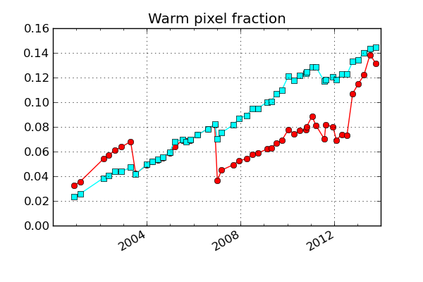
Note that the temperature assigned to a dark calibration is the mean of the temperature for the invidivual dark replicas (typically 5). These in turn use ACA hdr3 diagnostic telemetry for high-resolution temperature readouts which are available before and after (but not during) each replica.
Dark current modeling
This module will contain functions related to analytical models of the dark current as well as derived predictions of ACA guide and acquisition performance based on correlations with the warm pixel fraction. This is still in work, see mica.archive.aca_dark.dark_model.
Processing
This module updates the MICA ACA dark current archive when new dark current calibrations are completed. For details see the API documentation at mica.archive.aca_dark.update_aca_dark.
ACA diagnostic telemetry
The mica.archive.aca_hdr3 module works with Header 3 data (extended ACA diagnostic telemetry) available in 8x8 ACA L0 image data. The module provies an MSID class and MSIDset class to fetch these data as “pseudo-MSIDs” and return masked array data structures. See Header 3 Pseudo-MSIDs for the list of available pseudo-MSIDs.
>>> from mica.archive import aca_hdr3 >>> ccd_temp = aca_hdr3.MSID('ccd_temp', '2012:001', '2012:020') >>> type(ccd_temp.vals) 'numpy.ma.core.MaskedArray' >>> from Ska.Matplotlib import plot_cxctime >>> figure(figsize=(5, 3.5)) >>> plot_cxctime(ccd_temp.times, ccd_temp.vals, '.')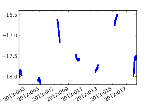 >>> perigee_data = aca_hdr3.MSIDset(['ccd_temp', 'aca_temp', 'dac'], ... '2012:125', '2012:155') >>> figure(figsize=(5, 3.5)) >>> plot(perigee_data['aca_temp'].vals - perigee_data['ccd_temp'].vals, ... perigee_data['dac'].vals, '.') >>> subplots_adjust(bottom=0.15) >>> ylabel('TEC DAC Control Level') >>> xlabel('ACA temp - CCD temp (C)')
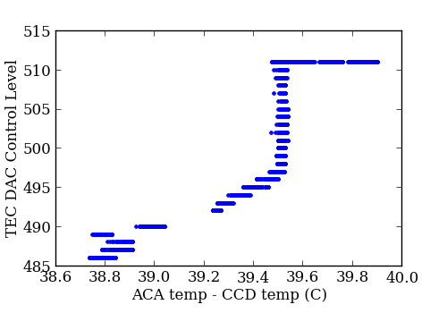
Retrieving pseudo-MSIDs with this module will be slower than Ska.engarchive fetches of similar telemetry, as the aca_hdr3 module reads from each of the collection of original fits.gz files for a specified time range. Ska.engarchive, in contrast, reads from HDF5 files (per MSID) optimized for fast reads.:
In [3]: %time ccd_temp = aca_hdr3.MSID('ccd_temp', '2012:001', '2012:020')
CPU times: user 5.18 s, sys: 0.12 s, total: 5.29 s
Wall time: 7.46 s

In [9]: %time quick_ccd = Ska.engarchive.fetch.MSID('AACCCDPT', '2012:001', '2012:020')
CPU times: user 0.02 s, sys: 0.00 s, total: 0.03 s
Wall time: 0.81 s
ACA L0 telemetry
The mica.archive.aca_l0 module provides tools to build and fetch from a file archive of ACA L0 telemetry. This telemetry is stored in directories by year and day-of-year, and ingested filenames are stored in a lookup table.
Methods are provided to retrieve files and read those data files into data structures.
>>> from mica.archive import aca_l0
>>> obsid_files = aca_l0.get_files(obsid=5438)
>>> time_8x8 = aca_l0.get_files(start='2011:001', stop='2011:010',
...                             imgsize=[8])
>>> time_files = aca_l0.get_files(start='2012:001:00:00:00.000',
...                               stop='2012:002:00:00:00.000',
...                               slots=[0], imgsize=[6, 8])
The values from those files may be read and plotted directly:
>>> from astropy.io import fits
>>> from Ska.Matplotlib import plot_cxctime
>>> figure(figsize=(5, 3.5))
>>> for aca_file in time_files:
...     f = fits.open(aca_file)
...     plot_cxctime(f[1].data['TIME'], f[1].data['TEMPCCD'], '.')
...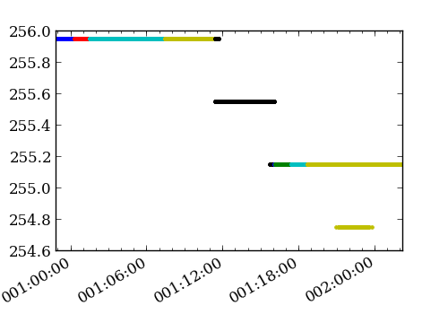
This particular loop/plot will break if the images aren’t filtered on “imgsize=[6, 8]”, as the ‘TEMPCCD’ columns is only available in 6x6 and 8x8 data. That’s one reason to use the convenience function get_slot_data(), as it places the values in a masked array (masking, for example, TEMPCCD when in 4x4 mode or when the data is just not available).
>>> temp_ccd = aca_l0.get_slot_data('2012:001:00:00:00.000',
...                                 '2012:002:00:00:00.000',
...                                  slot=0, imgsize=[6, 8],
...                                  columns=['TIME', 'TEMPCCD'])
>>> figure(figsize=(5, 3.5))
>>> plot_cxctime(temp_ccd['TIME'], temp_ccd['TEMPCCD'], '.')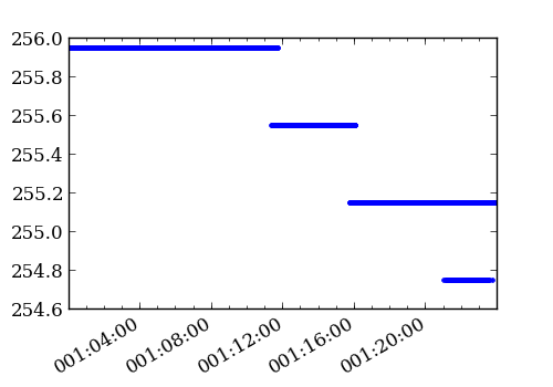
(it is still wise to filter on imgsize in this example, as there is no advantage to reading each of the 4x4 files.)
The get_slot_data() method will retrieve all columns by default and the resulting data structure, as mentioned, will have masked columns where those values are not available (i.e. HD3TLM64 in 6x6 or 4x4 image data). See ACA L0 MSIDs/columns for the list of available columns.
The aca_l0 archive includes all of the raw image data. The following code grabs the image data from slot 2 during a fid shift and creates a plot of each readout.
>>> from scipy.stats import scoreatpercentile
>>> from itertools import izip, count
>>> slot_data = aca_l0.get_slot_data(98585849, 98585884, slot=2)
>>> vmax = scoreatpercentile(np.ravel(slot_data['IMGRAW']), 98)
>>> vmin = scoreatpercentile(np.ravel(slot_data['IMGRAW']), 2)
>>> norm = mpl.colors.LogNorm(vmin=vmin, vmax=vmax, clip=1)
>>> for raw, idx in izip(slot_data['IMGRAW'], count()):
...     fig = figure(figsize=(4,4))
...     imshow(raw.reshape(8,8, order='F'),
...            interpolation='none',
...            cmap=cm.gray,
...            origin='lower',
...            norm=norm,
...            aspect='equal')
...     savefig("slot_2_{0:02d}.png".format(idx))
ImageMagick has been used to knit those plots together:
convert -delay 20 -loop 0 slot*.png slot_2.gif
to create this:
Aspect L1 products
The mica.archive.asp_l1 module provides tools to build and fetch from a file archive of Aspect level 1 products.
Methods are provided to find the archive directory:
>>> from mica.archive import asp_l1
>>> asp_l1.get_dir(2121)
'/data/aca/archive/asp1/02/02121'
>>> obsdirs = asp_l1.get_obs_dirs(6000)
The obsdirs dictionary should look something like:
{'default': '/data/aca/archive/asp1/06/06000',
2: '/data/aca/archive/asp1/06/06000_v02',
3: '/data/aca/archive/asp1/06/06000_v03',
'last': '/data/aca/archive/asp1/06/06000',
'revisions': [2, 3]}
Methods are also provided to retrieve a list files by obsid and time range.
>>> obs_files = asp_l1.get_files(6000)
>>> obs_gspr = asp_l1.get_files(6000, content=['GSPROPS'])
>>> range_fidpr = asp_l1.get_files(start='2012:001',
...                                stop='2012:030',
...                                content=['FIDPROPS'])
Observation parameters
The mica.archive.obspar module provides tools to build and fetch from a file archive of obspars.
Methods are provided to find the archive directory and obspar files:
>>> obspar.get_obspar_file(7000)
'/data/aca/archive/obspar/07/07000/axaff07000_000N002_obs0a.par.gz'
>>> obspar.get_dir(2121)
'/data/aca/archive/obspar/02/02121'
>>> obsdirs = obspar.get_obs_dirs(6000)
The obsdirs dictionary should look something like:
{'default': '/data/aca/archive/obspar/06/06000',
2: '/data/aca/archive/obspar/06/06000_v02',
3: '/data/aca/archive/obspar/06/06000_v03',
'last': '/data/aca/archive/obspar/06/06000',
'revisions': [2, 3]}
A method is provided to read the obspar into a dictionary:
>>> from mica.archive import obspar
>>> obspar.get_obspar(7001)['detector']
'ACIS-I'
Methods are also provided to retrieve a list of files by obsid and time range.
>>> obs_files = obspar.get_files(6000)
>>> range = obspar.get_files(start='2012:001',
...                          stop='2012:030')
Mica.stats
The mica.stats.acq_stats module includes code to gather acquisition statistics data for each observation and return those data to the user.
Access stats data
To get the whole acquisition table data:
>>> from mica.stats.acq_stats import get_stats
>>> stats = get_stats()
>>> stats[(stats['obsid'] == 5438) & (stats['slot'] == 1)][0]['dy']
8.4296239297976854
The hdf5 in-kernel searches may be faster working with the table directly for some operations.
Mica.VV
The mica.vv module provides tools to create and inspect V&V-type data
Access Mica V&V Data
Locate mica v&v products:
>>> from mica.vv import get_vv_dir
>>> get_vv_dir(16504)
'/data/aca/archive/vv/16/16504_v01'
List files:
>>> from mica.vv import get_vv_files
>>> get_vv_files(16504)
['/data/aca/archive/vv/16/16504_v01/vv_report.json',
 '/data/aca/archive/vv/16/16504_v01/vv_slot.pkl',
 '/data/aca/archive/vv/16/16504_v01/vv_report.pkl',
 '/data/aca/archive/vv/16/16504_v01/slot_0_yz.png',
 ...
Retrieve all residuals:
>>> from mica.vv import get_rms_data
>>> data = get_rms_data()
>>> data[data['obsid'] == 16505]['dz_rms']
array([  2.62251067e-05,   5.16913551e-02,   5.32668958e-02,
         4.78861857e-02])
Retrieve mica v&v values for an already-mica-processed obsid. The dictionaries of values still need more documentation at this time.
>>> from mica.vv import get_vv
>>> obs = get_vv(16504)
>>> obs['slots']['7']['dz_rms']
0.11610256063309182
Run mica V&V tools directly
Using the mica-archived aspect solution and obspar, run the mica obsid tools
>>> from mica.vv import get_arch_vv
>>> obi = get_arch_vv(2121)
Plot slot 4 residuals
>>> obi.plot_slot(4)
Look at the SIM drift values
>>> obi.info()['sim']
{'max_d_dy': 0.002197265625,
 'max_d_dz': 0.0018472671508789062,
 'max_medf_dy': 3.3234403133392334,
 'max_medf_dz': 7.3717021942138672,
 'min_medf_dy': 3.0496618747711182,
 'min_medf_dz': 6.3389387130737305}
The Obi class can also be called directly on data that isn’t in the mica archive. For example, on c3po-v, something like this could be used to plot residuals on un-ingested data (these directories will likely not exist to run this example in the future):
>>> proc_dir = '/dsops/ap/sdp.10/opus/prs_run/done/ASP_L1____502323245n674/'
>>> aspect_dir = proc_dir  + 'output'
>>> obspar = proc_dir + 'input/axaff14565_000N001_obs0a.par'
>>> import mica.vv
>>> obi = mica.vv.Obi(obspar, aspect_dir)