Using Contrib Color Look-Up Tables
CIAO 4.16 Science Threads
Overview
Synopsis:
Users can follow this thread if they wish to use the contributed color look-up tables in ds9, matplotlib, or dmimg2jpg.
Purpose:
One of the easiest customizations that users can do in CIAO is to use a non-standard color look-up table (LUT) or some times called color map.
Beyond the aesthetics of a particular color choice, different LUT's can be used to convey additional meaning: highlighting certain regions, emphasizing gradients, and provide additional reference between datasets.
This thread will show you how to load the contributed color look-up tables into ds9, matplotlib, and dmimg2jpg
Related Links:
- An inf@Vis article on the use of colour in cartography and visualisation, as championed by by Cynthia A. Brewer of Penn State, who created the ColorBrewer site.
- A follow-up article in inf@Vis on the spectral (or rainbow) palette, pointing out that the Rainbow Color Map (Still) Considered Harmful.
- mean_energy_map tool
- dmimg2jpg tool
- ds9 thread
Last Update: 13 Jan 2022 - Review for CIAO 4.14. No changes.
Contents
- Get Started
- Background Information
- Contributed Look-Up Tables
- How to Use Contributed LUT's
- History
- Images
Get Started
Download the sample data: 214 (CAS A)
unix% download_chandra_obsid 214 evt2
Background Information
Many different fields of science rely on different color look-up
tables (LUT's): medical
imaging, cartography, meteorology, fluid dynamics,
as well as astronomy. It is not surprising then that
there are many different color maps
available. The largest repository seems to be
cpt-city
which has 100's of different color maps from both the scientific
community as well as the realm of artistic/graphic-design. ds9
version 7 now has a direct link to cpt-city and all their color
maps are now available in ds9's .sao format.
The color map chosen is up to the user to decide based on what information they are trying to convey. For most scientific purposes, the only common restriction would be that colors are unique: having the color "white" show up at both a low intensity level and a high pixel intensity level in the color map may lead to ambiguity. This is not an absolute rule as one may choose to obscure certain regimes of the data with the same color to draw focus on a different area.
Examples of which color map to use when
If one were to have an image whose pixels represent the incident integrated flux, a colored gradient, one maybe chosen to symbolically match the energy band pass, may be a good choice (Figure 1 and Figure 2). An image showing temperatures is often shown using a rainbow color scheme (Figure 3). And an image showing color, that is the ratio of two images in different energy bands, may best be shown with a color map that smoothly varies between two colors (Figure 4).
Figure 1: Image of Low Energy Events
![[Thumbnail image: ]](ds9_loweng.png)
[Version: full-size]
Figure 1: Image of Low Energy Events
Figure 2: Image of High Energy Events
![[Thumbnail image: ]](ds9_higheng.png)
[Version: full-size]
Figure 2: Image of High Energy Events
Figure 3: Pseudo Temperature Map
![[Thumbnail image: ]](ds9_mean_energy.png)
[Version: full-size]
Figure 3: Pseudo Temperature Map
Figure 4: Hardness Ratio
![[Thumbnail image: ]](ds9_hr.png)
[Version: full-size]
Figure 4: Hardness Ratio
Contributed Look-Up Tables
These LUT's were extracted from two different software package and the data were reformatted to ds9's .lut format.
- HEAsoft's
XImage
package,
a multi-mission X-ray image display and analysis program
- National Institutes of Health's
ImageJ
package,
a public domain Java image processing program inspired by [National Institutes for Health] Image
.
Note: Some of these color maps may be identical or nearly identical to one or more of those already available in ds9, matplotlib, or dmimg2jpg
XImage
 Click on colorbars to see example. |
|
|
|
ImageJ
|
Click on colorbars to see example. |
|
|
|
How to Use Contributed LUT's
All the color look-up tables will be located in $ASCDS_CONTRIB/data. You can access them by name by using the ximage_lut.par and imagej_lut.par parameter files.
unix% plist ximage_lut

Parameters for /soft/ciao-4.4/contrib/param/ximage_lut.par

#
# Color Lookup Tables extracted from NASA XImage package
#
#    http://heasarc.gsfc.nasa.gov/xanadu/ximage/ximage.html
#
# converted to the ".lut" format used by ds9, chips, and dmimg2jpg
#
#
           (bb = ${ASCDS_CONTRIB}/data/bb.lut -> /soft/ciao-4.4/contrib/data/bb.lut) Color Lookup Table
        (blue1 = ${ASCDS_CONTRIB}/data/blue1.lut -> /soft/ciao-4.4/contrib/data/blue1.lut) Color Lookup Table
        (blue2 = ${ASCDS_CONTRIB}/data/blue2.lut -> /soft/ciao-4.4/contrib/data/blue2.lut) Color Lookup Table
        (blue3 = ${ASCDS_CONTRIB}/data/blue3.lut -> /soft/ciao-4.4/contrib/data/blue3.lut) Color Lookup Table
        (blue4 = ${ASCDS_CONTRIB}/data/blue4.lut -> /soft/ciao-4.4/contrib/data/blue4.lut) Color Lookup Table
  ...

unix% plist imagej_lut

Parameters for /export/ciao-4.4/contrib/param/imagej_lut.par

#
#
# Color Lookup Tables extracted from the NIH's ImageJ package
#
#  http://rsbweb.nih.gov/ij/
#
# converted to the ".lut" format used by ds9, chips, and dmimg2jpg
#
     (000-gray = ${ASCDS_CONTRIB}/data/000-gray.lut -> /export/ciao-4.4/contrib/data/000-gray.lut) Color Lookup Table
     (001-fire = ${ASCDS_CONTRIB}/data/001-fire.lut -> /export/ciao-4.4/contrib/data/001-fire.lut) Color Lookup Table
 (002-spectrum = ${ASCDS_CONTRIB}/data/002-spectrum.lut -> /export/ciao-4.4/contrib/data/002-spectrum.lut) Color Lookup Table
      (003-ice = ${ASCDS_CONTRIB}/data/003-ice.lut -> /export/ciao-4.4/contrib/data/003-ice.lut) Color Lookup Table
   ...
Using contributed LUT's in ds9
As with most things in ds9, there are at least 3 different ways to load a new color map: via the GUI, on the command line, and via XPA. Only the first two are shown here.
On the command line, you use the -cmap load command
unix% ds9 acisf00214N000_evt2.fits -cmap load $ASCDS_CONTRIB/data/heart.lut
Figure 5: ImageJ "heart" LUT in ds9
![[Thumbnail image: ]](ds9_casa_heart.png)
[Version: full-size]
Figure 5: ImageJ "heart" LUT in ds9
Alternatively, in the ds9 GUI, you can load the color map by going to Color -> Colomap Parameters ... In the sub-window, then go to File -> Load Colormap ..., navigate to the CIAO contrib/data directory and select the file name.
When a custom color map is loaded, it will be available under the top level "Color" menu. Prior to version 7, the name of the new color map would simply be appended to the list of those built-in. In version 7, custom color maps have their own sub-menu.
Using contributed LUT's in matplotlib
In this example we use the parameter module to retrieve the file name from the imagej_lut.par file. We then parse this file into the red, green, blue, and alpha (transparency) channels used by the ListedColormap class.
% python

import paramio as pio
from pycrates import read_file
import matplotlib.pylab as plt
from matplotlib.colors import ListedColormap

heart_lut = pio.pget("imagej_lut", "heart")
tab = open(heart_lut,"r").readlines()
rgb = [ x.strip().split() for x in tab if not x.startswith("#")]
rgba= [ [float(x[0]),float(x[1]),float(x[2]),1.0] for x in rgb ]
heart_lut_cmap = ListedColormap(rgba)

img = read_file('img_sm_asinh.fits')
imgvals = img.get_image().values
plt.imshow(imgvals, origin='lower', cmap=heart_lut_cmap)
plt.savefig("matplotlib.png")
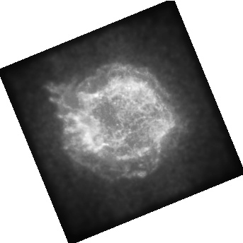
Figure 6: ImageJ "heart" LUT in matplotlib
![[Thumbnail image: ]](matplotlib.png)
[Version: full-size]
Figure 6: ImageJ "heart" LUT in matplotlib
The "heart" color look-up table from ImageJ being used in matplotlib. The input file was created by applying an asinh transform to a smoothed image from the event file using dmimgcalc.
Note: the data are shown in logical image pixel coordinates.
Using contributed LUT's in dmimg2jpg
The look-up table can be fed directly to dmimg2jpg. In the follow example we make use of a parameter redirect to locate the file name.
unix% dmimg2jpg infile=img_sm.fits outfile=img_sm.jpg \
  lutfile=")imagej_lut.heart" \
  scalefun=log mode=h clobber=yes
Figure 7: ImageJ "heart" LUT in dmimg2jpg
![[Thumbnail image: ]](dmimg2jpg_heart.png)
[Version: full-size]
Figure 7: ImageJ "heart" LUT in dmimg2jpg
History
| 10 Oct 2012 | Initial version. |
| 13 Dec 2012 | Review for CIAO 4.5; added note about adding color bar via chips gui and added several inf@Vis articles on the use of color to the Related Links section. |
| 24 Apr 2013 | To avoid a naming conflict, ximage.par and imagej.par have been renamed ximage_lut.par and imagej_lut.par |
| 25 Nov 2013 | Review for CIAO 4.6. |
| 16 Dec 2014 | Reviewed for CIAO 4.7; no changes. |
| 01 Feb 2016 | Updated ds9 links. |
| 29 Dec 2016 | Reviewed for CIAO4.9. No changes. |
| 28 Mar 2019 | Updated to use matplotlib. |
| 13 Jan 2022 | Review for CIAO 4.14. No changes. |