Joining Juno to Explore Jupiter's X-ray Emissions
W. Dunn, G. R. Gladstone, Z. Yao, D. Weigt, R. Kraft, G. Branduardi-Raymont, A. Wibisono, S. Kotsiaros, C. Jackman
We normally think of X-ray astronomy in the context of the unimaginably powerful and violent. The typical playgrounds for X-ray astronomers are neutron stars, black holes and exploding massive stars. At the grandest scales, X-ray astronomy enables our exploration of the evolution of the entire cosmos, revealing the connections between the largest gravitationally bound structures in the Universe—galaxy clusters. Given the profoundly different scales of energy and size, it may seem surprising that our relatively modest archetypal gas giant, Jupiter, is also a bright X-ray source (Figure 1). Why and how ‘a mere planet’ generates the energies required for X-ray production has remained unknown for four decades.
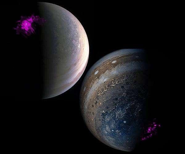
Figure 1: Overlaid Chandra HRC and Juno images of Jupiter’s pole. Top left shows a projection of Jupiter’s Northern X-ray aurora (purple) overlaid on a visible Junocam image of the North Pole. Bottom right shows the Southern counterpart [Credit: NASA Chandra/Juno Wolk/Dunn].
Yet, a closer look reveals that Jupiter is no ‘mere planet’. In fact, Jupiter’s X-ray emissions may be indicative of the superlatives that set it apart from the other planets. Besides containing more than twice the mass of the other planets of the solar system combined, Jupiter also possesses the strongest known planetary magnetic field, with a magnetic moment 20,000 times greater than Earths. Jupiter rotates the fastest and through this rapid-rotation its magnetic field is whipped through its surrounding space environment every 9.9 hours. A tug-of-gravitational-war between Jupiter and its other moons, causes Jupiter’s moon, Io, to be the most volcanic body in the solar system, injecting a ton of volcanic material (predominantly sulfur and oxygen) into space every second. This volcanic material becomes ionized and is picked-up by Jupiter’s rapidly rotating magnetic field and accelerated to rotate with the planet (to ‘corotate’), producing an environment around the planet in which the pressure from the hot plasma can exceed the pressure from Jupiter’s magnetic field by factors of 100. The combination of these factors fills the Jovian magnetosphere (the region of space controlled by Jupiter’s magnetic field) with particles from keV to GeV1 energies, bloating it to produce the largest coherent structure in the solar system. If the naked eye could see the Jovian magnetosphere, we would observe this 5 AU long structure (intermittently touching Saturn) stretching across the night sky to cover a region several times the size of our moon (Figure 2). The combination of these factors leads Jupiter to generate the brightest aurorae in the solar system, which can be used as a remote diagnostic of the processes governing the magnetosphere.
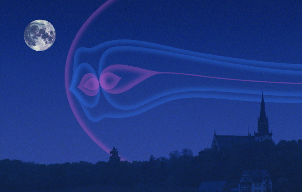
Figure 2: Illustration of the size of Jupiter’s magnetosphere if it could be seen by human eye in the night sky [Credit: NASA/ESA]
Many of the conditions present in the Jovian magnetosphere are local analogues for other astrophysical objects. The planet therefore provides a natural laboratory in which we can study the connection between remotely observed X-rays and the physical processes and conditions that produce them. For example, twisting and shearing of rapidly-rotating magnetic field lines informs processes occurring at other rapid rotators. While a comparison to magnetars and neutron stars may seem far-fetched for now, brown dwarfs and exoplanets are clearly reliant on understanding of Jupiter. Equally, the conditions (density, temperature, ratio of plasma to magnetic pressure) in the centrifugally-confined plasma disc that surrounds the planet are not greatly dissimilar to the plasmas present in galaxy clusters. However, unlike more exotic X-ray targets, Jupiter is an astronomical stone’s throw away, enabling exploration with in-situ spacecraft. Indeed, for X-ray astronomy, Jupiter’s proximity may prove to be one of its greatest assets.
Currently, NASA’s Juno spacecraft is orbiting Jupiter. This is offering a once-in-a-generation opportunity to compare observations by Chandra, XMM-Newton and NuSTAR with in-situ measurements of the physical conditions and processes that enable planets to produce X-ray emission. In this article, we: discuss the history of X-ray observations of Jupiter, present the rich variety of X-ray emissions that the planet, its moons and its surrounding space environment produce, show new simultaneous observations by Juno and X-ray instruments, and close with a look to what the future might bring.
A History of Jupiter's X-rays
Since the time of the Neanderthals, homo sapiens have gazed in wonder at the dazzling auroral light displays in Earth’s atmosphere. 30,000 years ago, our oldest ancestors engraved their fascination with these awe-inspiring phenomena into cave walls. Yet, it wasn’t until the second half of the 20th century that we first discovered aurorae on another world—Jupiter2.
In Spring 1979, the Einstein X-ray observatory detected the first X-ray emissions from another world – Jupiter’s dynamic X-ray aurorae (Figure 3)3. That same year, the Voyager spacecraft undertook their ground-breaking fly-bys of the gas giant and first observed Jupiter’s terawatt UV aurorae4—the brightest aurorae in the solar system. This laid the foundations for decades of synergistic high energy auroral observations.
Despite the relatively primitive spectral resolution offered by the Einstein Observatory’s Imaging Proportional Counter, the instrument showed that Jupiter’s X-ray aurorae was unlikely to be produced by electron bremsstrahlung3. Instead, the authors prophetically suggested that it may be produced by precipitating MeV ions—an idea that would take decades to confirm. The small-scale complementary X-ray
spacecraft that followed Einstein (e.g. EXOSAT and GINGA), were unsuitable for Jupiter observations, so X-ray studies of planets remained dormant for a decade, until ROSAT could observe the planet in the 1990s5–9.
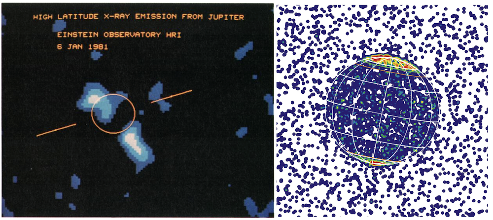
Figure 3: Left: Image of Jupiter as taken by the Einstein X-ray observatory High Resolution Imager in 19813. Right: The first Chandra HRC X-ray Image of Jupiter overlaid with a graticule mapping lines of latitude and longitude (white)10.
The temporal and spatial resolution offered by ROSAT first revealed that Jupiter’s X-ray aurorae were controlled by the planet’s tilted magnetic field, so that the Northern lights would rotate in and out of view each Jupiter rotation—a tenuous high energy analogy is perhaps an exceptionally slow pulsar (e.g. see movie/gif in Fig 4). Further, ROSAT uncovered a second X-ray emission at Jupiter: emission from the equatorial atmosphere, showing that Jupiter’s hydrogen-dominated atmosphere is excellent for scattering solar X-rays. In fact, Jupiter’s atmosphere can be used as a diagnostic of the X-ray spectrum from the entire solar disk11–15. The disk of Jupiter brightens, dims and changes spectra with changing solar X-ray emission over both the 12-year solar cycle15 and on ~minute timescales through solar-flares.
While the Einstein and ROSAT observations laid the firmest foundations, it was the launch of Chandra and XMM-Newton in 1999 that would revolutionize our understanding of planetary X-ray emissions. Their complementary capabilities have enabled a continuous stream of ground-breaking discoveries.
The very first Chandra X-ray image of Jupiter was taken in December 2000 (Figure 3) and provided a paradigm-shift in our understanding of Jupiter’s X-rays. The exquisite spatial and temporal resolution on the High Resolution Camera (HRC) enabled X-ray maps of Jupiter to be produced (e.g. Figure 5). These maps show a very different planet to the orange and grey striped world that we typically associate with visible images of Jupiter. Chandra’s spatial resolution has proved irreplaceable in characterizing a diverse array of X-ray emissions from Jupiter. For brevity, here we’ll focus on two structures in Jupiter’s X-ray aurora: Jupiter’s pulsing X-ray spots and the hard X-ray oval, but note that other X-ray sources also exist16.
Figure 4: gif/movie showing the X-ray aurora rotate in and out of view during a 10 hour Jupiter rotation. X-ray flares are observed to occur quasi-periodically every 45-minutes on top of this 10 hour rotational modulation [Credit: Gladstone] 10.
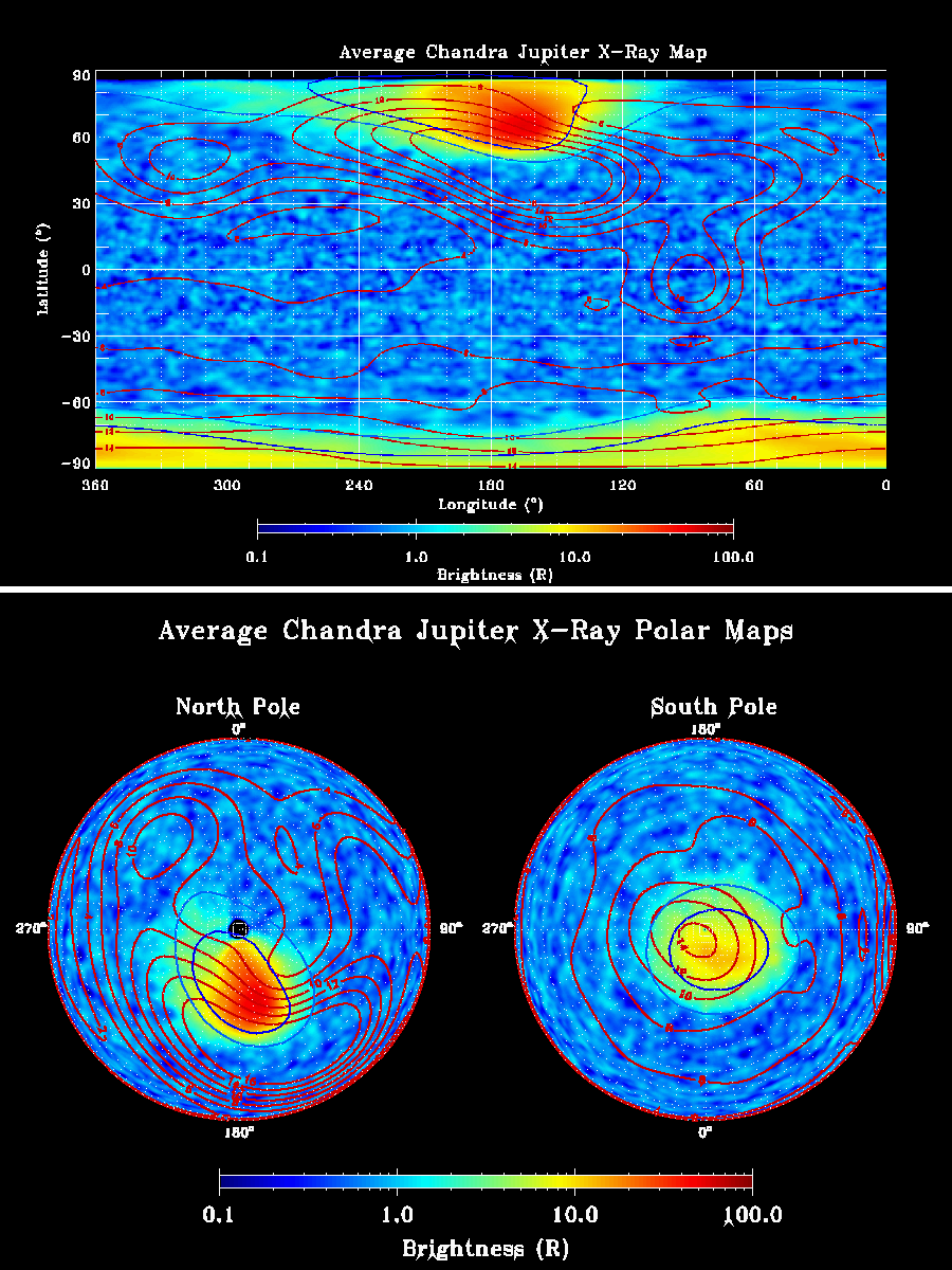
Figure 5: X-ray Maps of Jupiter. Top: Chandra X-ray Longitude-Latitude map of Jupiter from combining nearly all observations of the planet since 2017. Dashed lines indicate latitude and longitude coordinates in the planet’s System III coordinates. Bottom: Polar projections of Jupiter’s Northern (left) and Southern (right) X-ray aurorae. The outer blue contour shows the footprint of Jupiter’s satellite Io as it orbits the planet. Magnetic field lines in this region will map to an equatorial location that is 6 RJ (Jupiter radii) from the planet. The inner blue contour shows the location of Jupiter’s main auroral oval. Magnetic field lines along the main oval contour will map to an equatorial location 30 RJ. The red contours on the latitude-longitude and polar projection maps show the surface magnetic field strength at Jupiter’s surface as measured by Juno. The numerical values on these red contours show the magnetic field strength in Gauss.
Quasi-Periodic Flaring X-ray Aurora Hot Spots
The first Chandra observations revealed that much of Jupiter’s Northern X-ray aurora was concentrated into a bright ‘hot spot’ structure close to the magnetic pole10. Such X-ray aurora hot spots have now been seen at both poles15–19. Mysteriously, these hot spots often pulsate with a clockwork-like regular period10,19–22. Figure 6a shows an example from June 2016 when the Southern aurora pulsed every 9-13 minutes for multiple observations19. Strangely, the North and South sometimes pulse in time together21, but also often pulse out of sync. Normally the Southern aurorae is much dimmer than the Northern aurorae (e.g. see Figure 9). The reasons for the North-South independence remain unknown. Tracing the magnetic field lines in this region shows that these auroral flares were produced by explosive releases of energy millions of kilometers away from the planet, in its outer magnetosphere14,19,23.
Synchronized Chandra ACIS and Hubble Space Telescope observations have shown that the quasi-periodic X-ray flares coincide with bright ultraviolet aurora flares24, with powers of the order of terawatts. The spectral resolution provided by Chandra’s ACIS and XMM-Newton have shown that the X-ray flares are dominated by charge exchange lines from oxygen ions25,26 (e.g. O6+,7+; Figure 6b), along with other ion species that current energy resolution is yet to unambiguously identify.
Charge exchange occurs when ions collide with neutrals and ‘steal’ an electron from the neutral. If the ion is sufficiently highly charged then the relaxation of the electron to the lowest energy levels will produce an X-ray photon27. While X-ray emissions are often associated with hot environments, the charge exchange process enables X-rays to be leveraged for the study of the interface between hot plasma and cool neutral material. Jupiter’s charge exchange process occurs in a quite different context to the commonly discussed solar wind charge exchange, in which already highly charged solar wind ions (e.g. O7+,8+), collide with neutrals. This is commonly observed for the coma of comets28.
Rather than the solar wind, the dominant heavy ion source for Jupiter is likely to be the magnetosphere14,15,21,24,29–31, which has a plentiful supply of its own heavy ions of sulfur and oxygen, thanks to the volcanic eruptions on Io. While the ionization processes in Jupiter’s magnetosphere typically only permit the ions to reach states of up to ~O3+, sufficiently energetic (~MeV) ions will undergo further electron stripping when they precipitate into Jupiter’s atmosphere. These energetic collisions produce the O7+,8+ that generate the charge exchange lines observed31–38.
These energetic particle precipitations have broad ramifications for the planet, resulting, for example, in anomalous heating of the atmosphere39, which impacts the atmospheric chemistry of the planet. In fact, for Jupiter, the injections of auroral energy exceed the energy from solar radiation globally; making Jupiter’s aurorae a key driver of the atmospheric chemistry.
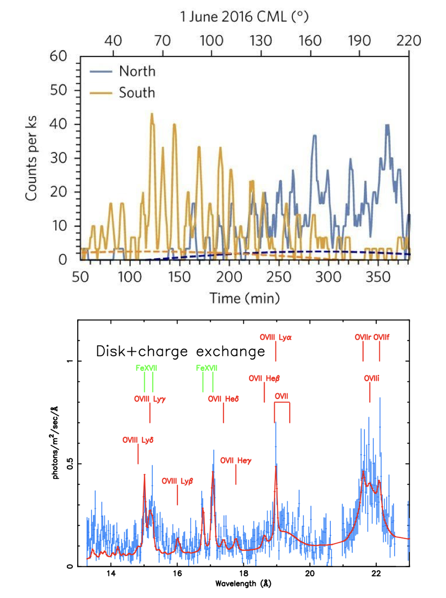
Figure 6, Top: Northern (blue) and Southern (gold) X-ray lightcurves from Jupiter on 1 June 2016, showing characteristic pulsing of emission every 9-13 minutes19. Jupiter’s longitude that would appear in the center of the planet for an observer on Earth (it’s Central Meridian Longitude – CML) is shown along the top of the plot. Lower: XMM-Newton RGS spectrum from Jupiter showing the oxygen charge exchange lines that dominate this wavelength range in Jupiter’s X-ray spectrum26.
The Hard X-ray Auroral Oval
Chandra ACIS has also showed that the pulsing soft X-ray (E < 2 keV) hot spot is encircled by an oval of hard X-ray (E > 2 keV) bremsstrahlung emission from precipitating electrons. Figure 7a shows that these precipitating electrons coincide with a bright UV auroral structure called Jupiter’s ‘main oval’ 40.
The source of this hard X-ray and UV auroral main oval is thought to be a global current system through which Jupiter imparts angular momentum into the surrounding magnetospheric plasma to keep it rotating with the planet41,42. This ‘co-rotation enforcement current’ flows with precipitating electrons at the UV/X-ray main oval carrying the upward (away from Jupiter) current. It has been suggested that the precipitating ions in the hot spot may carry (or trace) the returning (toward Jupiter) co-rotation current29 (figure 7b). If this is the case then this co-rotation enforcement current spans millions of kilometers across the Jovian magnetosphere. While Jupiter’s main oval is a quasi-continuous persistent structure, it brightens and dims significantly when perturbed by external shocks (such as those caused by the solar wind). The impact of these shocks on the space environment around Jupiter can be studied both in-situ and remotely through auroral observations.
The Influence of the Solar Wind on Jupiter
While Earth’s aurorae are governed by the solar wind, many of Jupiter’s auroral emissions may well exist with or without the presence of the solar wind. While the solar wind doesn’t drive Jupiter’s aurorae, solar storms such as coronal mass ejections that erupt from the Sun and collide with Jupiter’s magnetosphere can shock the system. These shocks rapidly compress Jupiter’s dayside magnetosphere by up to 30% perturbing the system and modulating the auroral emissions. The auroral X-ray, UV, IR and radio emissions are all observed to change during such shocks14,21,22,39,43–49. Figure 8 shows that for the X-rays, solar wind driven compressions of the magnetosphere change the auroral brightness, spatial and spectral morphology and trigger 25-35 minute X-ray pulsations 14,21,22.
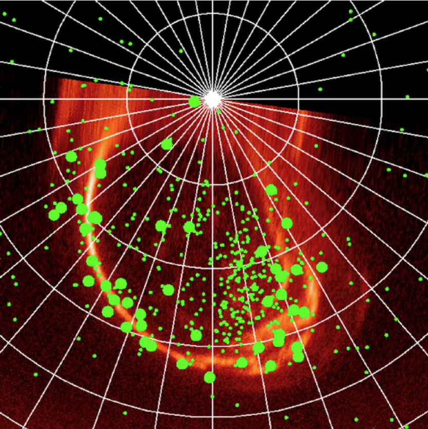
Figure 7: Left: North pole projection of Jupiter’s X-ray (green dots) and UV (orange) aurorae as observed by Chandra ACIS and the Hubble Space Telescope 40. Large dots show hard X-ray (E > 2 keV) photons from electron bremsstrahlung and small dots show soft (E < 2keV) X-ray photons from charge exchange emission from precipitating ions. White lines are lines of latitude and longitude in increments of 10 degrees. Right: Schematic of the global corotation enforcement current system that is thought to produce Jupiter’s hard X-ray and UV main emission at the footpoint of the upward current50 and applies a J × B force to the magnetospheric plasma to accelerate it towards corotation.
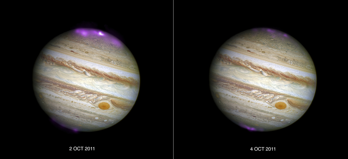
Figure 8: Two Chandra ACIS observations of Jupiter’s X-ray aurorae overlaid on a Hubble image of the planet. On October 2nd 2011 a solar storm (an interplanetary coronal mass ejection) impacted Jupiter causing the aurora to expand, brighten and change spectral and temporal morphology, with regularly pulsed auroral flares. By October 4th 2011 the solar storm had subsided and the magnetosphere was recovering from the shock. During this interval the aurora was dimmer, smaller and pulsing more slowly14 [Credit: NASA].
So what produces Jupiter’s X-ray aurorae and why/how does Jupiter produce these diverse emissions when other planets (e.g. Saturn51) do not? An array of processes have been proposed: reconnection of magnetic field lines along the magnetopause30, the global co-rotation enforcement current system29, reconnection in Jupiter’s plasmadisk 52,53 or Kelvin Helmholtz instabilities along the magnetopause14,19,23. To test these possibilities required remote observations to be connected with in-situ measurements. With Juno, we are now in an era when this testing and a potential subsequent resolution is possible.
Jupiter's X-rays in the Juno Era
37 years after the ground-breaking discoveries of the Voyager spacecraft and Einstein Observatory, the rare opportunity to again combine in-situ measurements of Jupiter with remote X-ray observations arrived when NASA’s Juno spacecraft entered orbit around Jupiter in Summer 201654. Juno’s orbital trajectory takes the spacecraft to never before explored regions. Its 53-day daredevil orbits take the spacecraft from ~5000 km above the cloudtops at the poles to the furthest regions of the magnetosphere and the boundary with the solar wind.
The combination of Juno’s orbit and its suite of particle55,56, magnetic field57 and multi-waveband58 remote sensing instrumentation including radio, microwave, IR, visible and UV instruments, mean the spacecraft is ideally suited to probe the causes of X-ray emission at Jupiter. However, Juno doesn’t possess an X-ray instrument—in fact, a soft X-ray detector has never visited the outer planets.
Over the past 3 years a set of unparalleled Jupiter X-ray campaigns have been conducted that leverage the unique opportunity that Juno presents. This has meant months of planning to connect Juno’s orbit with Chandra, XMM-Newton and NuSTAR’s visibility, so that observations can be taken precisely when Juno is exploring in-situ processes in the relevant magnetospheric locations for X-ray emissions. It is a huge tribute to the fantastic operations teams from these instruments, that such datasets now exist, providing a rich and irreplaceable legacy of observations, which will be invaluable for decades to come. The planetary X-ray community is unanimously grateful for the extensive support of the operations teams.
Connecting, calibrating and correlating X-ray emissions from the planet with in-situ magnetic field and particle measurements ranging from locations directly above the aurorae, to distances millions of kilometers from the planet has proven exceptionally challenging, but this year the first results of these correlations have begun to be published21,22,38. Here, we highlight some preliminary results of coordinated X-ray-Juno simultaneous observations to demonstrate the rich array of possibilities presented through these multi-instrument datasets. We also recommend interested readers to look-out for several new results that are currently under embargo.
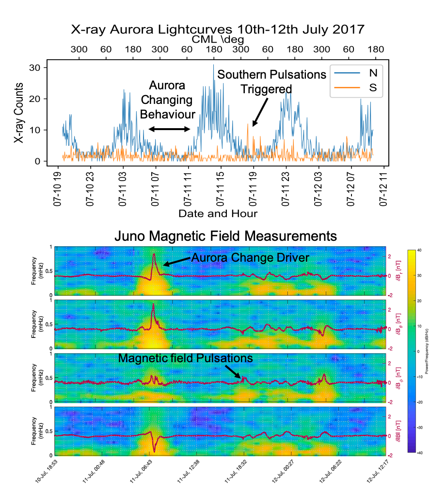
Figure 9: Top: X-ray lightcurves from Jupiter’s Northern (blue) and Southern (yellow) aurora during a 40 hour XMM-Newton EPIC-pn observation from July 10-12th 2017. CML across the top of the plot indicates the line of Jupiter longitude facing Earth at a given time. The Northern auroral behavior changes between the aurora rotating out of view at 06:30 on July 11th and rotating back into view at 11:00 on July 11th. Lower: Juno magnetic field measurements from the MAG instrument. Power spectral density is shown with the color bar, while the change in magnetic field from the ambient magnetic field strength is shown in red for magnetic field coordinates r, theta, phi and the total magnetic field, respectively. Arrows indicate magnetic field behaviors that drive the X-ray auroral signatures shown above.
Figure 10: gif/movie: Polar projections of Jupiter’s Northern and Southern X-ray aurorae, during a series of observations in July 2019. Grey lines indicate 10 degree increments in latitude and 45 degree increments in longitude. (Click image to play movie)

Figure 11: Spectrogram of heavy ion (sulfur and oxygen) fluxes on 16 May 2017 from the Juno JEDI instrument. These show pulsations in the ion fluxes on 20-30 minute time scales.
Figure 9 shows a comparison between X-ray lightcurves for Jupiter’s Northern and Southern aurora and Juno magnetic field measurements from the 10-12 July 2017. The Northern aurora can be seen to rotate in and out of view 5 times. Between 07:00 and 11:00 on 11 July 2017, Jupiter’s X-ray aurora mysteriously switches behavior. By inspecting the Juno in-situ observations at this time it is possible to identify a sharp change in the magnetic field at ∼08:00. This spike is thought to be from a magnetic field reconfiguration in which the topology of Jupiter’s magnetic field lines changes. One example of such phenomena is when stretched magnetic field lines undergo a process called magnetic reconnection, which allows part of the field line to ‘snap off’ (often explosively)52,53,59. Having shed this tension, the magnetic field then returns to a more dipole-like structure. To inspect this possibility further, a campaign of Chandra observations was organized in July 2019, when Juno was ideally located to measure further changes. Figure 10 shows variability in the X-ray aurora during the expected several day cycle of Jupiter’s magnetic field topology changing.
A little later during the observation on 11 July 2017, after 10:00, Juno moved into the Southern hemisphere magnetosphere. The Southern X-ray aurorae is generally dim and inactive throughout this observation until 18:00 on 11 July, when it begins pulsing. Just prior to these X-ray pulsations, Jupiter’s Southern hemisphere magnetic field lines also begin to exhibit pulsations. The pulsation rate for the magnetic field and the X-ray aurorae is the same (a pulse every 42.5 minutes), showing the deep connection between the two. Figure 11 shows that similar pulsations are also often seen in in-situ ion data observed by Juno’s JEDI instrument.
So what physical processes produce Jupiter’s pulsating X-ray hot spot? The answer was not what we had expected. Comparisons between the in-situ data and the X-ray aurora reveal a chain of connections from global dynamics to small-scale particle responses. These show that perturbations to the planet’s magnetic field cause the plasma distributions to change. When this happens the plasma responds by producing waves that cause MeV ions to be directed along the magnetic field towards the planet to produce Jupiter’s X-ray aurora. The perturbations and subsequent plasma response are intermittent (e.g. Figure 9 magnetic field pulsations), which leads the X-ray flares to be intermittent. Further details and simultaneous datasets are under embargo but will hopefully be published later this year in Yao et al. [in review] and Dunn et al. [in review].
Beyond in-situ comparisons, multi-waveband observations can also be connected. Figure 12 (13) shows gifs of overlaid simultaneous Chandra observations and Juno UVS (Hubble Space Telescope) images obtained when Juno flies directly over the pole of Jupiter, highlighting the link between the X-rays and the UV ‘active region’. With the physical context for some X-ray emissions now known, it is possible to re-interpret these photon-rich UV observations.
Figure 12a/b: gif/movie: Chandra observations of X-ray photons (blue stars) from Jupiter’s Northern (left) and Southern (right) aurorae overlaid on simultaneous Juno UVS observations of the UV aurorae during flights over the pole. The yellow arc shows the direction of the Sun. The multi-colored pig-tail-like contour shows the footprint of the Juno spacecraft as it flew over the pole. The color bar on this shows the energy flux of precipitating oxygen as measured by the Juno JEDI instrument during this flight [Gladstone et al. in prep].
Figure 13: Scenes from a movie (click image to play movie) of an overlay of a 45-minute North Pole Projection of Jupiter’s Northern UV and X-ray aurorae from Hubble (blue-white color bar) and Chandra (white dots) in 1 minute time steps for a 4-minute moving window. (Click image to play movie)
X-rays from Jupiter's Radiation Belts, Io Plasma Torus and Galilean Satellites
Beyond Jupiter itself, the Jovian space environment contains a rich and diverse set of X-ray sources. X-rays have provided direct observations of Jupiter’s radiation belts, where Suzaku observed inverse-Compton scattering by ultra-relativistic particles 60,61. Chandra observations have characterized emission from the Io Plasma torus, where non-thermal bremsstrahlung emission and oxygen fluorescence and/or charge exchange produce X-rays62. However, arguably the most exciting X-ray sources in the system are the Galilean satellites: Io, Europa and Ganymede. X-ray fluorescence has been used to study the composition of our own moon since the Apollo era63 and, more recently, the planet Mercury through NASA’s Messenger spacecraft64 and soon through ESA-JAXA’s BepiColombo65. For these bodies, fluorescence is caused by the impact of solar photons with atoms in the surface of the body. For Jupiter, the moons are too distant for solar irradiance to play a key role, instead impacts from the magnetospheric plasma cause the surface material to fluoresce62 (Figure 14). Chandra ACIS observations of the moons show spectral lines indicative of the surface composition (e.g. oxygen fluorescence from water ice on Europa).
The implications for such observations are profound. Understanding the elemental composition of the surface ice on Europa has key implications for chemistry in the subsurface oceans and any potential astrobiology. Unfortunately, Chandra’s ACIS instrument, which provided proof-of-concept fluorescence line identification, now has too much contaminant built-up on the detector at the key wavelengths, but this has laid firm foundations for studies with future instrumentation.
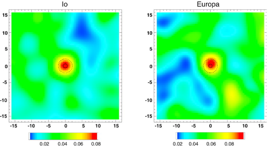
Figure 14. ACIS images of Io and Europa (250 eV < E < 2000 eV) from Elsner et al. [2002]. The images have been smoothed by a two-dimensional Gaussian with = 2’’ (5 ACIS pixels). The axes are labeled in arcsec (1’’ = 2995 km), and the scale bar is in units of smoothed counts per image pixel (0.492’’ × 0.492’’).
The Future of Planetary X-ray Studies
The future of planetary X-ray studies is exceptionally bright. In the near term (2021-), Juno will begin exploring Jupiter’s dusk sector, where the X-ray hot spot source is expected to be14,19,22,23. Chandra and XMM-Newton observations coincident with Juno’s exploration of this sector would determine if planetary X-rays are signatures of global or only localized processes.
Looking to the coming decades, ATHENA and potentially Lynx will provide step-changes. ATHENA will open X-ray investigations of the ice giants, Uranus and Neptune, while its X-IFU (X-ray Integral Field Unit – the cryogenic spectrometer) will deliver the extended wavelength range, and improved effective area that will enable unambiguous identification of the other ion species at Jupiter.
With 30 times the effective area of Chandra and the energy-dispersive resolution of a micro-calorimeter, the notional Lynx X-ray Observatory would also open entirely new avenues of investigation. Lynx observations of the aurora would provide spectrally resolved images of the variability of the ion aurora to rival the photon-rich UV videos shown from electron precipitation in the Hubble observations (e.g. Figure 13). Critically, the combination of Lynx’s spatial and spectral resolution would enable deep observations of the Galilean moons to determine the major elemental constituents of their surfaces.
Closer to home, development of the European Space Agency and Chinese Academy of Sciences’ SMILE mission (launch: 2023) will leverage X-ray charge exchange emissions along Earth’s magnetopause to study the global response of our own magnetosphere to space weather and the solar wind. This will provide the first global images of a magnetosphere.
In the outer solar system, an in-situ X-ray instrument akin to the Soft X-ray Imager on SMILE would be a game-changer. The current Jupiter X-ray results are based on observations that contain ~10s (for Io/Europa) to ~1000s (for Jovian aurora) of counts. An in-situ X-ray instrument would receive 7 orders of magnitude more flux, enabling a paradigm-shift in the science accomplished. For Jupiter’s moons, this would provide rich maps of the elemental composition of the surfaces, enabling regional analysis of astrobiological potential. Recent work has developed suitable fluorescence models applicable to the outer planet’s moons66, so that feasibility and instrument requirements can also be considered for moons like Enceladus at Saturn, Ariel at Uranus or Triton at Neptune.
This rich array of planetary X-ray possibilities is built on the revolutionary insights that Chandra and XMM-Newton have provided over the past 2 decades. These foundations have enabled fields of planetary science that would not otherwise exist and could not have been dreamt of 21 years ago. Future observations will undoubtedly continue to be essential for our understanding of our local neighborhood; the only astrophysical X-ray sources for which remote observations can be anchored to their in-situ sources.
Bibliography
1. Roussos, E. et al. The in-situ exploration of Jupiter’s radiation belts (A White Paper submitted in response to ESA’s Voyage 2050 Call). arXiv Prepr. arXiv1908.02339 (2019).
2. Burke, B. F. & Franklin, K. L. Observations of a variable radio source associated with the planet Jupiter. J. Geophys. Res. 60, 213–217 (1955).
3. Metzger, A. E. et al. The detection of X rays from Jupiter. J. Geophys. Res. 88, 7731 (1983).
4. Broadfoot, A. L. et al. Extreme ultraviolet observations from Voyager 1 encounter with Jupiter. Science (80-. ). 204, 979–982 (1979).
5. Waite, J. H. et al. ROSAT observations of the Jupiter aurora. 99, 799–809 (1994).
6. Waite, J. H. et al. Equatorial X-ray emissions: Implications for Jupiter’s high exospheric temperatures. Science (80-. ). 276, 104–108 (1997).
7. Waite, J. H. et al. ROSAT observations of X-ray emissions from Jupiter during the impact of comet Shoemaker-Levy 9. Sci. YORK THEN WASHINGTON- 1598 (1995).
8. Gladstone, G. R., Waite, J. H. & Lewis, W. S. Secular and local time dependence of Jovian X ray emissions. J. Geophys. Res. Planets 103, 20083–20088 (1998).
9. Gladstone, G. R. et al. Equatorial X-ray Emissions?: Implications for. 276, (1997).
10. Gladstone, G. R. et al. A pulsating auroral X-ray hot spot on Jupiter. Nature 415, 1000–1003 (2002).
11. Branduardi-Raymont, G. et al. Latest results on Jovian disk X-rays from XMM-Newton. Planet. Space Sci. 55, 1126–1134 (2007).
12. Bhardwaj, A. et al. Low- to middle-latitude X-ray emission from Jupiter. J. Geophys. Res. Sp. Phys. 111, 1–16 (2006).
13. Bhardwaj, A. et al. Solar control on Jupiter’s equatorial X-ray emissions: 26-29 November 2003 XMM-Newton observation. Geophys. Res. Lett. 32, 1–5 (2005).
14. Dunn, W. R. et al. The impact of an ICME on the Jovian X-ray aurora. J. Geophys. Res. A Sp. Phys. 121, (2016).
15. Dunn, W. R. et al. Jupiter’s X-rays 2007 Part 1: Jupiter’s X-ray Emission During Solar Minimum. J. Geophys. Res. Sp. Phys.
16. Dunn, W. R. et al. Jupiter’s X-ray Emission 2007 Part 2: Comparisons with UV and Radio Emissions and In-Situ Solar Wind Measurements. J. Geophys. Res. Sp. Phys.
17. Elsner, R. F. et al. Simultaneous Chandra X ray, Hubble Space Telescope ultraviolet, and Ulysses radio observations of Jupiter’s aurora. J. Geophys. Res. Sp. Phys. 110, (2005).
18. Branduardi-Raymont, G. et al. Spectral morphology of the X-ray emission from Jupiter’s aurorae. J. Geophys. Res. Sp. Phys. 113, (2008).
19. Dunn, W. R. et al. The independent pulsations of Jupiter’s northern and southern X-ray auroras. Nat. Astron. 1, (2017).
20. Jackman, C. M. et al. Assessing Quasi-Periodicities in Jovian X-Ray Emissions: Techniques and Heritage Survey. J. Geophys. Res. Sp. Phys. 123, (2018).
21. Wibisono, A. D. et al. Temporal and Spectral Studies by XMM-Newton of Jupiter’s X-ray Auroras During a Compression Event. J. Geophys. Res. Sp. Phys.
22. Weigt, D. M. et al. Chandra Observations of Jupiter’s X-ray Auroral Emission During Juno Apojove 2017. J. Geophys. Res. Planets 125, (2020).
23. Kimura, T. et al. Jupiter’s X-ray and EUV auroras monitored by Chandra, XMM-Newton, and Hisaki satellite. J. Geophys. Res. Sp. Phys. 121, 2308–2320 (2016).
24. Elsner, R. F. et al. Simultaneous Chandra X ray Hubble Space Telescope ultraviolet, and Ulysses radio observations of Jupiter’s aurora. J. Geophys. Res. Sp. Phys. 110, 1–16 (2005).
25. Branduardi-Raymont, G., Elsner, R. F., Gladstone, G. R. & Ramsay, G. First observation of Jupiter by XMM-Newton. Astronomy 337, 331–337 (2004).
26. Branduardi-Raymont, G. et al. A study of Jupiter’s aurorae with XMM-Newton. Astron. Astrophys. 463, 761–774 (2007).
27. Cravens, T. E., Howell, E., Waite, J. H. & Gladstone, G. R. Auroral oxygen precipitation at Jupiter. J. Geophys. Res. Sp. Phys. 100, 17153–17161 (1995).
28. Cravens, T. E. Comet Hyakutake x-ray source: Charge transfer of solar wind heavy ions. Geophys. Res. Lett. 24, 105–108 (1997).
29. Cravens, T. E. et al. Implications of Jovian X-ray emission for magnetosphere-ionosphere coupling. J. Geophys. Res. Sp. Phys. 108, (2003).
30. Bunce, E. J., Cowley, S. W. H. & Yeoman, T. K. Jovian cusp processes: Implications for the polar aurora. J. Geophys. Res. Sp. Phys. 109, 1–26 (2004).
31. Hui, Y. et al. Comparative analysis and variability of the Jovian X-ray spectra detected by the Chandra and XMM-Newton observatories. J. Geophys. Res. Sp. Phys. 115, n/a—n/a (2010).
32. Kharchenko, V., Dalgarno, A., Schultz, D. R. & Stancil, P. C. Ion emission spectra in the Jovian X-ray aurora. Geophys. Res. Lett. 33, 1–5 (2006).
33. Kharchenko, V., Bhardwaj, A., Dalgarno, A., Schultz, D. R. & Stancil, P. C. Modeling spectra of the north and south Jovian X-ray auroras. J. Geophys. Res. Sp. Phys. 113, 1–11 (2008).
34. Hui, Y. et al. The ion-induced charge-exchange X-ray emission of the Jovian Auroras: Magnetospheric or solar wind origin? Astrophys. J. Lett. 702, L158 (2009).
35. Ozak, N., Schultz, D. R., Cravens, T. E., Kharchenko, V. & Hui, Y.-W. Auroral X-ray emission at Jupiter: Depth effects. J. Geophys. Res. Sp. Phys. 115, (2010).
36. Ozak, N., Cravens, T. E. & Schultz, D. R. Auroral ion precipitation at Jupiter: Predictions for Juno. Geophys. Res. Lett. 40, 4144–4148 (2013).
37. Houston, S. J., Ozak, N., Young, J., Cravens, T. E. & Schultz, D. R. Jovian Auroral Ion Precipitation: Field-Aligned Currents and Ultraviolet Emissions. J. Geophys. Res. Sp. Phys. 123, 2257–2273 (2018).
38. Houston, S. J. et al. Jovian Auroral Ion Precipitation: X-Ray Production from Oxygen and Sulfur Precipitation. J. Geophys. Res. Sp. Phys.
39. Sinclair, J. A. et al. A brightening of Jupiter’s auroral 7.8-?m CH
40. Branduardi-Raymont, G. et al. Spectral morphology of the X-ray emission from Jupiter’s aurorae. J. Geophys. Res. Sp. Phys. 113, 1–11 (2008).
41. Hill, T. W. The Jovian auroral oval. J. Geophys. Res. 106, 8101–8107 (2001).
42. Cowley, S. W. H. & Bunce, E. J. Origin of the main auroral oval in Jupiter’s coupled magnetosphere-ionosphere system. Planet. Space Sci. 49, 1067–1088 (2001).
43. Prangé, R. et al. An interplanetary shock traced by planetary auroral storms from the Sun to Saturn. Nature 432, 78–81 (2004).
44. Baron, R. L., Owen, T., Connerney, J.E. P, Satoh, T., Harrington, J. Solar Wind Control of Jupiter ’ s H 3 Auroras. Icarus 442, 437–442 (1996).
45. Zarka, P. Auroral radio emissions at the outer planets: Observations and theories. J. Geophys. Res. Planets 103, 20159–20194 (1998).
46. Southwood, D. J. & Kivelson, M. G. A new perspective concerning the influence of the solar wind on the Jovian magnetosphere. J. Geophys. Res. Sp. Phys. 106, 6123–6130 (2001).
47. Chané, E., Saur, J., Keppens, R. & Poedts, S. How is the Jovian main auroral emission affected by the solar wind? J. Geophys. Res. Sp. Phys. 122, 1960–1978 (2017).
48. Nichols, J. D., Clarke, J. T., Gérard, J. C., Grodent, D. & Hansen, K. C. Variation of different components of jupiter’s auroral emission. J. Geophys. Res. Sp. Phys. 114, 1–18 (2009).
49. Clarke, J. T. et al. Response of Jupiter’s and Saturn’s auroral activity to the solar wind. J. Geophys. Res. Sp. Phys. 114, (2009).
50. Mauk, B. H. & Saur, J. Equatorial electron beams and auroral structuring at Jupiter. J. Geophys. Res. Sp. Phys. 112, 1–20 (2007).
51. Branduardi-Raymont, G. et al. Search for Saturn’s X-ray aurorae at the arrival of a solar wind shock. J. Geophys. Res. Sp. Phys. 118, 2145–2156 (2013).
52. Guo, R. L. et al. Reconnection Acceleration in Saturn’s Dayside Magnetodisk: A Multicase Study with Cassini. Astrophys. J. Lett. 868, (2018).
53. Guo, R. L. et al. Rotationally driven magnetic reconnection in Saturn’s dayside. Nat. Astron. 2, (2018).
54. Bolton, S. J. et al. Jupiter’s interior and deep atmosphere: The initial pole-to-pole passes with the Juno spacecraft. Science (80-. ). 356, 821–825 (2017).
55. Mauk, B. H. et al. The Jupiter energetic particle detector instrument (JEDI) investigation for the Juno mission. Space Sci. Rev. 213, 289–346 (2017).
56. McComas, D. J. et al. The Jovian auroral distributions experiment (JADE) on the Juno Mission to Jupiter. Space Sci. Rev. 213, 547–643 (2017).
57. Connerney, J. E. P. et al. The Juno magnetic field investigation. Space Sci. Rev. 213, 39–138 (2017).
58. Kurth, W. S. et al. The Juno waves investigation. Space Sci. Rev. 213, 347–392 (2017).
59. Vasyliunas, V. M. Plasma distribution and flow. Phys. Jovian Magnetos. 395–453 (1983).
60. Ezoe, Y. et al. Discovery of diffuse hard X-ray emission around Jupiter with Suzaku. Astrophys. J. Lett. 709, L178 (2010).
61. Numazawa, M. et al. Suzaku observation of Jupiter’s X-rays around solar maximum. Publ. Astron. Soc. Japan 71, 93 (2019).
62. Elsner, R. F. et al. Discovery of soft X-ray emission from Io, Europa, and the Io plasma torus. Astrophys. J. 572, 1077 (2002).
63. Adler, I. et al. Results of the Apollo 15 and 16 x-ray fluorescence experiment. Lunar Sci. IV, Ed. by JW Chamberlain C. Watkins 9 (1972).
64. Nittler, L. R. et al. The major-element composition of Mercury’s surface from MESSENGER X-ray spectrometry. Science (80-. ). 333, 1847–1850 (2011).
65. Fraser, G. W. et al. The mercury imaging X-ray spectrometer (MIXS) on bepicolombo. Planet. Space Sci. 58, 79–95 (2010).
66. Nulsen, S. et al. X-ray emission from Jupiter’s Galilean moons: A tool for determining their surface composition and particle environment. J. Geophys. Res. Sp. Phys.