
Soon after release of the new gain calibration (Jun 2020, CALDB 4.9.2) it was discovered that the LETG/HRC-S background filter was sometimes removing more than the intended 1% of valid X-ray events. A revised calibration was prepared (Jun 2021) and was released in CALDB 4.9.6. See here for details.
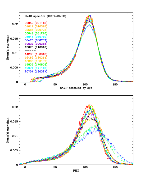
The purpose of a gain map is to obtain, for any given X-ray energy, identical pulse height distributions (PHDs) from all areas of the detector at all times. A simple linear scaling of the PHDs does a pretty good job, but as described in section 3.4 of the 2008 gain calibration, a more complicated equation is required to account for energy dependent gain effects, which were seen across all three HRC-S plates in pre-flight laboratory flat field data. That calibration worked well for several years, including right after the March 2012 high voltage change to restore the HRC-S QE and gain, but by around 2015, when detector gain was down to less than half what it was during lab calibration, the adjustments for energy dependence were causing significant distortions to the gain-adjusted PHDs (see bottom panel). Since there is no practical way to recalibrate the energy dependent effects using flight data, this new (2019/2020) calibration reverts to simple linear adjustments, which provide adequately consistent PHD shapes even at very low gains (top panel).
The new calibration benefits from several improvements over the 2008 calibration, of which the most important are:
The primary practical result of the gain calibration is that pulse height filtering can be applied to LETG spectra as a function of dispersed wavelength in order to reduce background by over half longward of 20 Å, compared with standard Level 2 processing.
Gain changes during flight are monitored by measuring pulse height amplitudes over time, using data from frequently observed continuum sources. HZ 43 covers longer wavelengths, mostly on the outer plates. PKS 2155 (up to 2008) and Mkn 421 cover shorter wavelengths, mostly on the inner plate. Calibration around the plate gaps has larger uncertainties because emission from all three sources is relatively weak at those wavelengths (roughly 50-70 Å).
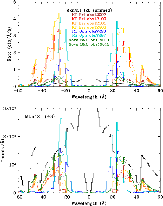
PKS 2155 and Mkn 421 spectra have significant contamination
from higher order diffraction, which shifts PHDs
to higher channels than for pure 1st order emission.
These effects can be modeled, but in order to check the accuracy
of our corrections we also analyze data from three bright novae,
RS Oph, KT Eri, and Nova SMC 2016,
that have emission over relatively narrow wavelength ranges
with minimal higher order contamination.
Over 30 observations of HZ 43 were used for this work,
nearly 40 of Mkn 421, and about two dozen of the other sources.
Spectra are shown in Figs. 1-3.

|
|
| |
| Fig. 1: [pdf] HZ 43 spectrum. | Fig. 2: [pdf] Mkn 421 spectra through June 2017, normalized to rates at 45 Å, showing spectral shape variations. | Fig. 3: [pdf] Spectra of Mkn 421, RS Oph, KT Eri, and Nova SMC 2016. The last three sources are largely free of higher orders, unlike PKS 2155 and Mkn 421. |
All data were reprocessed from Level 1 to Level 2 using the updated (May 2017, CALDB 4.7.4) HRC-S BADPIX file. All evt1 columns were retained (including RAWX and RAWY), and the SAMP column was added. SAMP is a cleaner version of PHA, defined as SAMP=SUMAMPS*(2.0^(AMP_SF-1.0))/128.0, and is used as the basis for PI and its various intermediate forms that we use in our analysis; it was added to Pipeline-processed data beginning in mid 2019.
After removing any periods of elevated detector background, spectra and background are extracted using narrower than usual regions designed to minimize background contamination. To characterize the detector gain at a given time and detector location we compute medians of the background-subtracted PHDs, usually binning data by 1/3 of a CRSV tap.
The HRC-S gain varies over time, and in order to
apply a time-independent pulse-height filter we must
calibrate the time dependence for each subtap.
As noted above, higher orders (HOs) contribute significantly to the spectra
of Mkn 421 and PKS 2155 at all but the shortest wavelengths.
We account for HO effects
by determining each order's flux as f(λ)
and modeling the measured PHD median as the flux-weighted
average of each order's median, using the previously calibrated
median vs λ relationship.
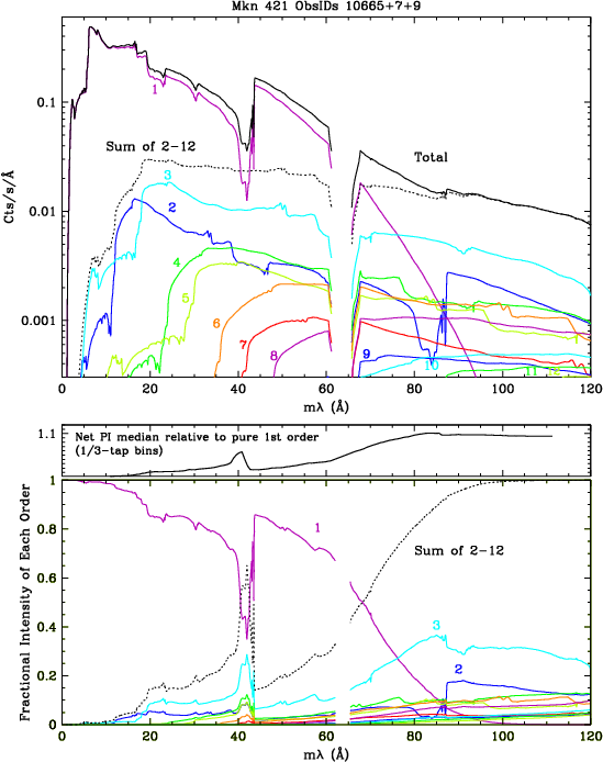
The magnitude of HO
corrections for one of the harder Mkn 421 spectra
is shown in the short middle panel of Figure 4.
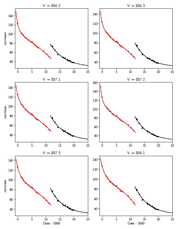
Corrected medians are then fitted with smooth curves
as a function of time (Figure 5), and the resulting gain corrections
are tabulated by epoch as TGAIN coefficients (Figure 6).
|
|

|
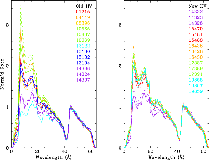
| Fig. 4: [pdf] Top: Fits to 12 +orders of Mkn 421 combined ObsIDs 10665,10667,10669. Middle: Ratio of measured and pure 1st order medians. Bottom: Relative contributions of each order. | Fig. 5: Fits to HO-corrected data (only 1st page shown). [87-page pdf]. Data for 98abc, 99abc, 100a are interpolated. | Fig. 6: [pdf] Gains for the 18 CALDB epochs (top panel for old HV, bottom for new), normalized to the gain in 2001.5. The green curve in the top panel is for 2001.22, when gains are close to those during lab calibration, and the blue curve in the bottom panel is the gain around the time of this time-dependence calibration (Jan 2020). Bottommost curve is for Oct 2 2022. Additional epochs can be added as necessary. |
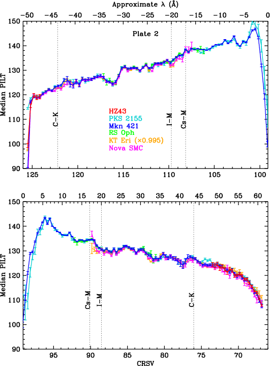
After applying the TGAIN corrections, multiple observations from the same source can be combined to improve statistical quality of the spatial calibration. PHD medians are again computed for each CRSV subtap, and count-weighted HO corrections are applied as needed. Results for the center HRC-S plate are shown in Figure 7. PHD median should vary smoothly as a function of wavelength, but it does not, especially near the ends of each plate. The observed spatial gain variations are the result of spatially non-uniform changes in gain that occurred between pre-flight lab calibration and our adopted mid-2001 reference gain.
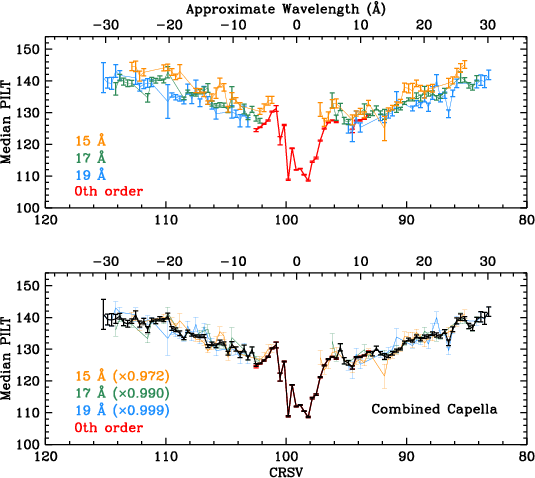
To calibrate the lab-to-flight spatial gain changes near the aim point we used several off-axis LETG observations of the emission-line source, Capella, spanning a range of Yoffset from -3.0' to +3.0'. By extracting 0th order and individual bright emission lines (around 15, 17 and 19 Å) we performed a set of "flat-field-like" calibrations, covering a nearly continuous range from CRSV=83 to 114 (Figure 8).
|
|
|
|
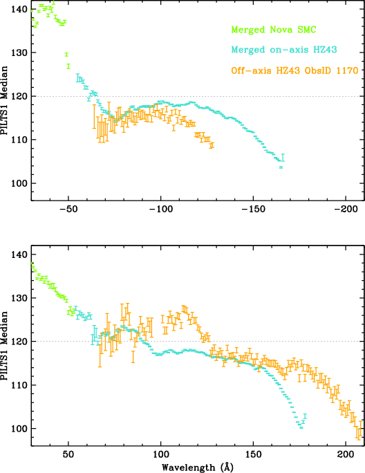
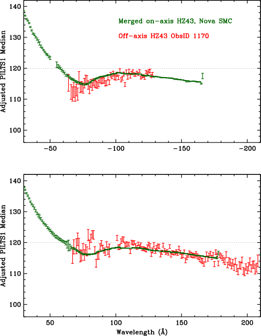
| Fig. 7: [Pdfs for plate3, 2, 1] Median PILT vs CRSV subtap on center plate using merged data, with HO corrections. | Fig. 8: [pdf] On- and off-axis Capella data used for gain "flat fielding." Top: Medians from Capella 0th order and bright lines. Bottom: Rescaled medians and combined curve for Capella. | Fig. 9: [pdf] PILTS1 medians for on- and off-axis spectra. The curves do not overlap because of incorrect relative gains on different areas of the detector. | Fig. 10: [pdf] Like Fig. 9 but after gain adjustments. |
Other regions of the detector can be calibrated, somewhat indirectly, by analyzing ObsID 1170, a 10-ks LETG/HRC-S observation of HZ43 made with Yoffset=10'. That offset corresponds to 17.80 taps, or a shift of 32.9 Å, allowing one to compare PHDs from a given wavelength at two widely separated locations on the HRC-S. As an example, in Fig. 9, the bump in the on-axis-observation curve around +70-95 Å is tied to the off-axis bump around 100-125 Å; both ranges correspond to CRSV of 61 to 49. Figures 9 and 10 show results before and after the gain adjustments.
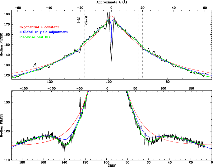
The revised spatial scaling is then applied, PHDs are extracted, and medians are computed. Results are shown in Fig. 11. The green curve is a piecewise fit using an exponential plus constant, modified with an empirical scaling factor based on the photocathode's CsI photoelectron yield. That final spatial gain calibration is used to create the CALDB GAINMAP. Figure 12 shows SAMP medians as function of time and wavelength, computed by rescaling model median vs λ using TGAIN and GAINMAP coefficients.
|

|
| Fig. 11: [pdf] Median PILTS2 vs CRSV, with various smooth curves. An exponential plus constant (red curve) follows the general shape. Adding a term based on the CsI photocathode's electron yield improves the fit; the blue curve shows best fits to the + and - orders (fitted separately). The green curve is a composite of results from fits over spans of typically 25 taps. | Fig. 12: [pdf] Modeled median SAMP for dispersed 1st order spectra, calculated using model PI medians (green fitted curve in Fig. 11) and rescaled using TGAIN and GAINMAP coefficients. |
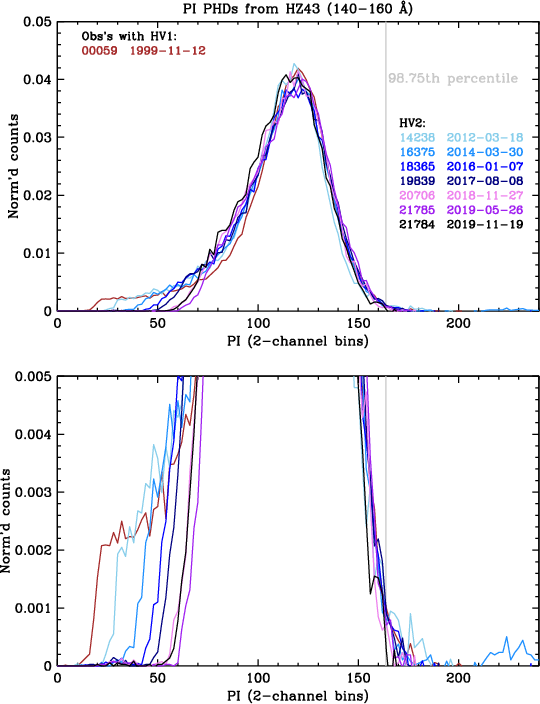
The ultimate purpose of this gain calibration is to allow processing of LETG/HRC-S data so that pulse height filtering can be applied, resulting in substantial background reduction with the loss of a very small and well determined fraction of X-ray source events. This requires that the shape of PI PHDs remains essentially constant over time, particularly at the high channels where filtering is applied. Figure 13 shows the PI PHDs from several HZ 43 observations over the course of the mission, around +150 Å where the detector gain is currently the lowest. As can be seen, the shape of the PI PHD at high channels changes very little over time.
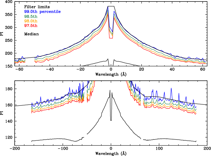
To determine the appropriate filtering limits, we extracted 1-Å bins from the merged source event files computed PI medians and high percentile metrics (97.5th to 99th), and applied HO corrections. Results are shown in Fig. 14. To construct the PI filter we chose to approximately follow the 99th percentile curve, which allows an adequate margin for time- and space-dependent variations in gain and PHD shape.
|
|
|

|
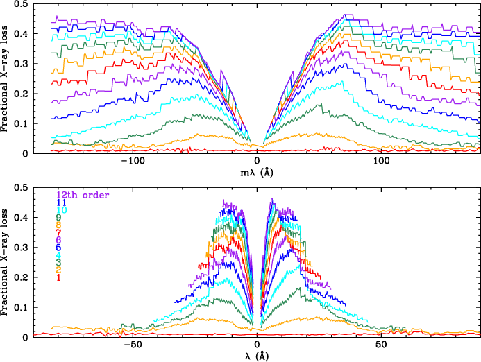
| Fig. 13: [pdf] PI PHDs for 140-160 Å, currently the lowest-gain region of the HRC-S. For clarity, only one observation with HV1 is shown. | Fig. 14: [pdf] Curves for the PI median and 97.5th to 99.0th percentiles. Top black curve denotes the PI vs tg_mlam filter, removing approximately 1.0 [0.8-1.5] percent of Level 2 X-ray events. | Fig. 15: [pdf] Effect of filtering on orders m=1-12. Curves are higher than true from ~12 to 17 Å because of small but increasing HO contamination in the Mkn 421 data used out to |λ|=17 Å; there is no real jump between 17 and 18 Å. The small step around 20 Å is caused by an increase in gain at the I-M absorption edge. The jump around 2 Å is also from photocathode absorption edges. | Fig. 16: [pdf] Effect of filtering on pure background in or near the spectroscopy region. Top: The most effective filtering is at long wavelengths, where events beyond PI~160 are removed (see Fig. 14). Bottom: Background PHD, with filtering limits at selected wavelengths. |
The 1% X-ray event loss is for the 1st order spectrum. Losses are progressively larger for higher orders, which have PHDs shifted to higher channels. Using the PHDs extracted from ~pure 1st order spectra, we applied the PI filter limits (for Å) to the PHDs for Å/m to determine the effect on mth order. Results through 12th order are shown in Fig. 21. Small losses of higher order flux will usually be unimportant, but observers can use Fig. 21 to estimate the effect of filtering on HOs and adjust their spectral fitting models accordingly.
To quantify the effect of filtering on background events we use data from ObsID 9617, in which the source was offset from the standard aim point by nearly 2 CRSU taps, leaving the standard spectroscopy region free of X-ray events. We extracted events from that region, applied the filter, and computed the fraction of events that remained after filtering (red points in top panel of Fig. 22). To obtain better statistics, we did the same analysis using a wider extraction region (black points). 60-70% of evt2 background events are removed at |λ|>40 Å, falling to ~20% removal at the shortest wavelengths.
The particle background varies over the solar cycle (see POG Fig. 9.21.) ObsID 9617 was collected in 2008, when the solar cycle was near its minimum, background rates were near their peak, and the cosmic ray energy distribution near Earth was somewhat harder (with relatively more background events at high channels) than at solar maximum. The background filter effectiveness shown in Fig. 37 therefore represents the best case. The fraction of background events that are removed by the filter near solar maximum (next expected ~2024) is a little lower, but the absolute background rate is also lower.
The current TGAIN calibration runs through fall 2022, but can be extended by adding more epochs and extrapolating the current fits, or by analyzing new data and making new fits. It is not unlikely that the detector high voltage will be increased within the next few years, which will of course require new TGAIN data. The decision on when to raise the voltage will be driven mostly by consideration of the decreasing QE.
Last modified: 06/16/20

