
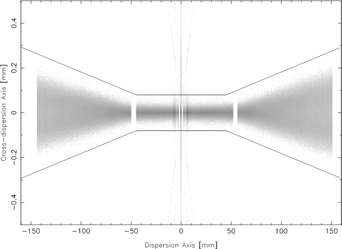
The LETG/HRC-S spectral extraction region has a 'bow tie' shape, narrow in the middle and widening on the outer plates to accommodate the inherent astigmatism of the LETG's Rowland-circle geometry. The shape and size of this region were chosen early in the mission based on MARX simulations (see Fig. 1) to roughly optimize the tradeoff between inclusion of X-ray signal versus particle background. The actual distribution of dispersed events, however, is somewhat different from the idealized simulations (e.g., Fig. 2). Using data collected over the past 15 years we have measured the cross-dispersion profiles of dispersed spectra as a function of wavelength, recalibrated the enclosed energy fractions (EEFRACs) tabulated in the CALDB LSFPARM files, and defined a narrower extraction region that improves the spectral S/N.
Most LETG/HRC observers will still want to use the standard bowtie extraction region because the improvement in S/N only becomes significant for very long exposures (>~100 ks) when studying weak features (S/N<~3). The net LETG/HRC effective area also remains unchanged as a result of this work because of compensating changes in the HRC-S QE. For those who wish to improve the S/N of their spectra we describe below a set of analysis threads, scripts, and files that will allow the user to:
|
|
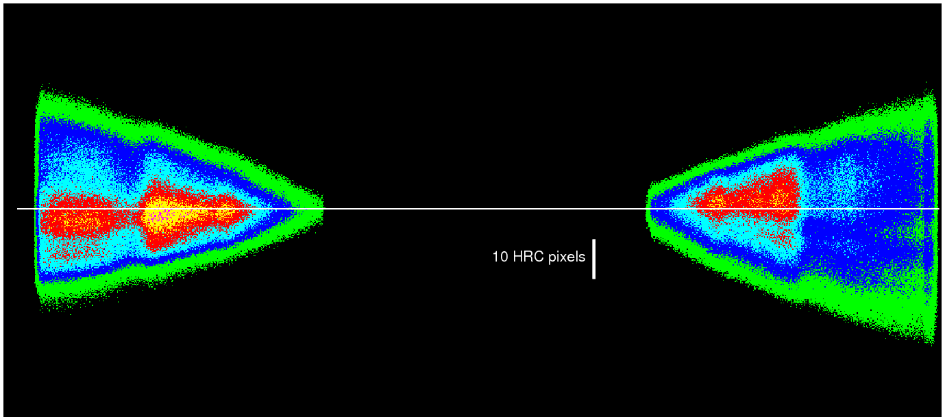
| Fig. 1. MARX simulation (c. 2000) of a flat spectrum illustrating the broadening of the LETG/HRC-S profile in the cross-dispersion direction toward longer wavelengths, and showing the standard bowtie extraction region. Vertical axis is stretched by a factor of ~220. | Fig. 2. Image of combined HZ43 spectra, after removal of tilts and wiggles (see below). Vertical axis is stretched by a factor of 200. The white horizontal line marks the median of the cross-dispersion profile, which is visibly asymmetric. |
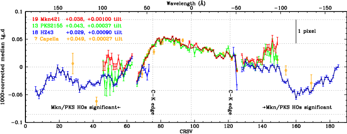
We used bright, frequently observed continuum sources to provide complete wavelength coverage with high signal, principally Mkn421 and PKS2155 for short wavelengths (<~60 Å) and HZ43 for longer wavelengths. We binned each spectrum by tap along the dispersion axis (crsv), subtracted background, and measured the median of the cross-dispersion profile (a.k.a. Line Spread Function, or LSF). After measuring and correcting for a slight tilt in each observation (Fig. 5) we observed a fixed pattern of wiggles (Fig. 4), which was also removed.
|
|
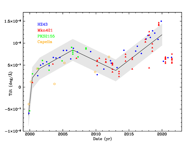
| Fig. 4. Median tg_d values for combined spectra, with tilt and offset adjustments to make the wiggle symmetric about tg_d=0. tg_d values are multiplied by 1000 for convenience and units are degrees. Tilts are in units of degrees per tap, also multiplied by 1000. Legend example: blue points are for 18 combined HZ43 spectra, with a tilt correction of 0.00090 and offset of 0.029. The composite wiggle curve is shown in black; some points near 0th order and the ends of the inner plate were adjusted by hand because the true errors are larger than indicated by the purely statistical error bars. (Clicking on the figure shows a 2-panel plot; the lower panel plots the same data without the offsets, showing the net wiggle correction and residual scatter among the different source curves.) | Fig. 5. Time dependent tilts deg/Å. Uncertainties on each point (excluding Capella) are small, so the observed scatter is real and probably related to thermal conditions. There is no apparent correlation with aimpoint jumps. The solid black line can be used to estimate the tilt in most observations, and the gray band denotes the degree of uncertainty that would cause a 1-pixel error at 170 Å. (This figure is updated roughly once a year.) |
Those same corrections were then applied to several observations
of two other sources used in the next step,
calibrating the cross-dispersion profile as a function of wavelength.
The additional sources, RS Oph and KT Eri, supplement the data
from Mkn421, whose profiles are affected at some wavelengths
by contributions from higher orders,
especially short of the C-K absorption edge at 44 Å.
The profiles were then used to calculate cumulative count
fractions as f(tg_d) (Fig. 11), including the contributions of
cross-dispersion orders diffracted by the LETG fine-support structure
(Fig. 10).
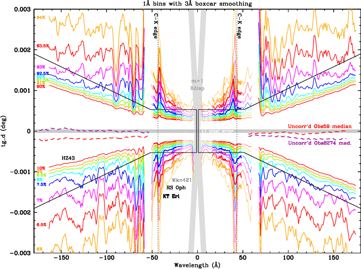
As seen in Fig. 11, the contours of cumulative count fractions are very noisy in the profile wings. Much of this comes from faint off-axis sources and nonlinearities in the detector background, primarily in regions outside the plotted tg_d range. Most of these background errors are excesses which tend to pull the contours away from the core. We can largely correct for this by forcing the outermost contours in our analysis, the 6% and 94% levels, to follow idealized contours. Note also in Fig. 11a that the contours for RS Oph and KT Eri are tighter than for Mkn421, which has higher order contamination that broadens the profiles.
The cleaned count fraction contours are plotted in Fig. 11b. After applying one last tg_d correction to make the profiles more symmetric about tg_d=0 (see Fig. 12 for the unadjusted profiles) we calculate new enclosed energy fractions (EEFRACs) for the CALDB LSFPARM file by interpolating our measured profiles, and scaling MARX-simulated profiles (at short wavelengths) and/or drawing smooth connecting curves where measurement errors become too large. We also use a finer grid of tg_d's in the new EEFRACS table (23 values instead of 10) to better capture the profiles' structure.
| 
|
| Fig. 11a. Cumulative count fractions from four continuum sources. Overlapping data on the center plate are distinguished by line thickness. The cross-dispersion 1st order is shown in light gray (seen as the faint "whiskers" in Fig. 1). Solid black lines mark the standard bowtie extraction region. The red and magenta "Uncorrected" curves show the medians for two ObsIDs with extreme tilts (before correction--see Fig. 3). The gray band in the middle has a half-width of 1 pixel; residuals after tilt and wiggle corrections are typically ±0.5 pixels or less. | Fig. 11b. "Corrected" version of Fig. 11a including more contours in the LSF core and using only the best data for the central plate, forcing the 6% and 94% contours to follow their assumed true values, and then drawing piecewise linear curves for all contours. Contours short of ~6 Å are approximate; final EEFRAC results at short wavelengths incorporate MARX modeling of Xdisp orders and scattering. |
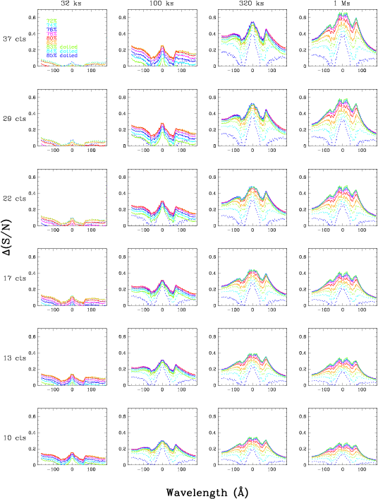
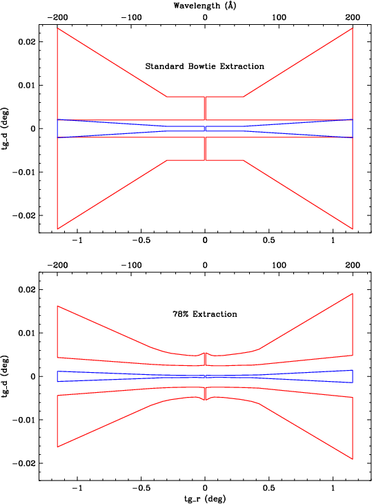
The standard bowtie extraction region is fairly conservative and using a narrower region generally yields better S/N, particularly for weak spectral features. The drawback of a narrower region is that errors in the spectral extraction efficiency become more sensitive to the exact positition and cross-dispersion profile of the spectrum, but these can be minimized by applying the corrections for 0th order, tilts, and wiggles. Fig. 14 plots the improvement in S/N for various combinations of spectral feature counts, exposure, and EEFRAC. We find that an extraction efficiency of ~78% (the standard bowtie region has an EEFRAC of ~86%) enerally provides the best S/N, although the improvement is usually not worth the extra effort of applying all our corrections unless the exposure time is very long and/or very weak features are being studied.

| 
|
| Fig. 12. tg_d profiles (0.00002-deg = 0.47-pixel bins) for 10-Å slices of the combined HZ43 spectrum. | Fig. 14. Change in S/N compared with using the standard bowtie extraction region. The optimal extraction region varies slightly depending on exposure, number of spectral feature counts, and wavelength but S/N is generally at or near its maximum with EEFRAC=78%. |
|
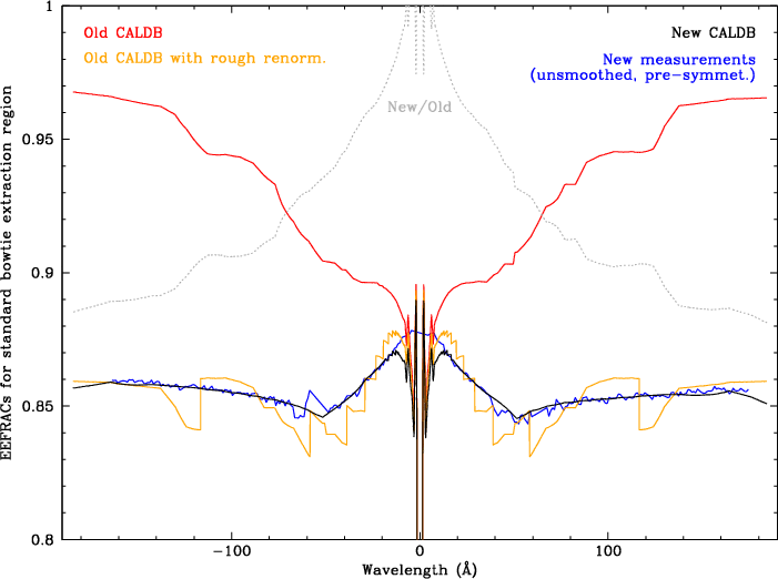
| Fig. 16. EEFRACs for the standard bowtie extraction region using data from the old CALDB data (red), roughly rescaled CALDB data (orange), calibration measurements (blue, using data from Fig. 11e), and new CALDB (black). The ratio of new and old CALDB EEFRACs (and he inverse of new vs old HRC-S QE) is shown in gray. |
The new EEFRAC tables, which were implemented in CALDB version 4.6.9 on 23 Sep 2015, are, strictly speaking, only appropriate when the full complement of tg_d corrections (tilt, wiggle, and symmetrization) is applied to the data, as should be done whenever a narrow extraction region is used. Errors in the derived EEFRAC are, however, negligible when using standard processing data (i.e., with the standard bowtie extraction region, without any tg_d corrections).
The EEFRACs from this work differ from those in the previous version of the CALDB because of deviations from the simulated LSF, 2% lower Xdisp intensity, and the previous incorrect normalization of flux to the detector area rather than to 2π. The net change in bowtie-region EEFRACs is typically several percent, and about 12% at the longest wavelengths (Fig. 16). Note that the overall absolute uncertainty in the LETG/HRC-S EA is unchanged at approximately ±10% (somewhat larger at long wavelengths because of complications from recent changes in HRC-S gain and QE). Uncertainties in the EEFRAC calibration are estimated to be 1-2% at most wavelengths, not including any errors in the Xdisp order calibration.
Despite these changes in the EEFRAC calibration, the net LETG/HRC-S effective area (EA) remains unchanged. This is because the EA, which includes the bowtie EEFRAC and HRC-S QE as factors, is calibrated by comparison with theoretical model spectra of Sirius B and PKS 2155/Mkn 421, so that any changes in EEFRACs are compensated by corresponding inverse changes in detector QE. The LETG/ACIS spectral extraction region is relatively wide so changes in the LSF near the core have little effect on the extraction efficiency and no changes are planned for the LETG/ACIS-S EA, which is based on absolute calibration of the grating efficiency, spectral extraction efficiency, ACIS QE, OBF transmission, and OSIPs (see LETG Calibration Overview).
LETG/HRC-S effective area remains unchanged for spectra extracted using the default bowtie region. For exposures of less than roughly 100 ks the choice of extraction region has a tiny effect on S/N and the default bowtie is fine. If, however, users are studying very weak features (S/N <~3) in long exposures and wish to maximize S/N they should:
Each step is described in detail below.
After downloading data from the archive the first step in the thread is to
Generate a New Level=1.5 Event File beginning with running
tg_create_mask.
As noted above, however, errors of a few tenths of a
pixel in 0th order are common in Archive data so
users must first determine the 0th order position manually.
Start with the position found by tgdetect and recorded
in the *evt1_src1a.fits file (and also in the region block
of the evt2.fits file).
dmlist "evt1_src1a.fits[srclist][cols pos]" data
(or
dmlist "archive_evt2.fits[region][#row=1][cols sky]" data)
This prints the coordinates of the 0th order (x0,y0) which can be used
as input to dmstat, running on either the evt1.fits or
evt2.fits file:
dmstat "archive_evt1.fits[(x,y)=circle(x0,y0,12)][cols sky]" | grep mean
Iteration of the above step is rarely necessary but is recommended
to confirm convergence.
(Note that off-axis observations may require a larger circle for
accurate centroiding.)
The improved 0th order coordinates (x0,y0)
are then used as input parameters to tg_create_mask,
following the thread but adding the lines
pset tg_create_mask use_user_pars=yes
pset tg_create_mask sA_zero_x=x0
pset tg_create_mask sA_zero_y=y0
before running tg_create_mask. (The input_pos_tab parameter will be ignored if specified; don't worry.) The thread continues with tg_resolve_events and then applies the pulse-height background filter, status filter, and GTI filter. The last step in the thread before extracting the grating spectrum is running hrc_dtfstats (see below).
Before running hrc_dtfstats users may want to examine DeadTime Factor (DTF) values by using chips to make a plot like Figure 1 in the Computing Average HRC Dead Time Corrections thread. Normally, DTF is larger than 0.98 but when telemetry is saturated during periods of high background or variable source emission it can be much less. One can filter out such times to reduce the average background and/or improve the livetime calculation accuracy, but this also removes all of the X-ray signal during those times and there is usually little if any benefit to the spectral S/N. More information about how to identify and remove periods of high background is presented here.
The commands discussed below are provided as part of the
Contributed Scripts
package of CIAO (release 4, Sep 2015) which includes
ahelp
documentation. To check your local CIAO installation's package
version type
ciaover -v | grep Contrib
The first step is to remove the wiggles (see Fig. 4) with
dewiggle uncorrectedEVT2.fits dewiggled.fits
This leaves a straight spectrum but usually one with a slight tilt that can be estimated from Fig. 5.
Tilt is removed with
   detilt dewiggled.fits detilted.fits
<tilt, e.g., 5.5e-7>
The last step is to apply the symmetrization correction so that
the EEFRAC file will yield an accurate extraction efficiency.
symmetrize detilted.fits ready2extract.fits
Note that only tg_d values are modified by these steps; spectra will still have tilts and wiggles in other coordinate systems, such as sky. Residual errors on tg_d in the detilted file should be no more than about 0.5 pixels on the central plate and 1.5 near the ends of the outer plates. All these tg_d corrections can be applied to off-axis observations but the CALDB EEFRACs only apply to on-axis observations; LSFs will, of course, be broader (and the true EEFRACs lower) for off-axis observations.
pset tgextract infile=ready2extract.fits
pset tgextract inregion_file=region78ee.fits
The custom region file also defines a new background region that uses the same value of BACKSCAL as the bowtie (5, for both the upper and lower BG region; see Fig. 19).
Processing then continues with the "HRC Grating RMFs" thread, picking up at "Run mkgrmf". The grating Response Matrix Files (gRMFs) that are generated by the thread (one for each order desired) incorporate the appropriate EEFRACs for the new region. The last step before fitting the spectrum is to generate the ARFs for each order, starting at the "Compute the Aspect Histograms" step of the "LETG/HRC-S Grating ARFs" thread.
|
| Fig. 19. Standard bowtie and optimized EEFRAC=78% extraction regions for spectra and background. Total background area is 10 times the spectral area in both cases. The optimized regions are not symmetric for - vs + wavelengths (c.f. Fig. 11). |
Last modified: 02/14/21

