HETGS Line Profiles

Validation: Wavelength

Wavelength

As mentioned earlier, we utilize four generic functions (2 Gaussians and 2 Lorentzians) to parameterize a line profile. The position of each function generally follows the trend described by the grating equation,

$m\lambda = p\ sin\beta$ where m is the integer order number, $\lambda$ is the photon wavelength in angstroms, p is the spatial period of the grating lines, and $\beta$ is the dispersion angle. However, small deviation from the grating relation may occur, as we freely manipulate the four functions to describe line profiles at any wavelengths. Hypothetically speaking it is plausible that the dominant Gaussian component may be shifted off-center slightly and then compensate the shift by altering both amplitude and position of one (or 2) of Lorentzian components, or vice versa. Hence we need an additional higher order polynomial fit to compensate such fluctuation.

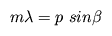
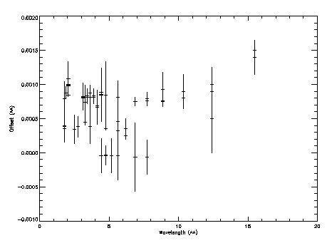
For each of the four functions, the centroid position is derived in the dispersion angle (in radian). At a very small angle, the dispersion angle is proportional to the wavelength value. So we fit a linear function to the angle-vs.-wavelength trend and then derive the scale of deviation of data points from the linear trend. The deviation points are fitted with piece-wise quadratic functions in order to ensure continuity on position and slope at each junction defined by the measured data points (see Figures 7 and 8 for the results of the fitting). Then later this non-linear term is added to the linear function to complete the analysis.

Scale of deviation of the measured wavelength from the linear trend (HEG)

Figure 7: The Scale of deviation of the measured positions from the linear grating relation (for HEG +1 order). Gaussian (titled as "G1P" and "G2P") and Lorentzian components ("L1P" and "L2P" likewise) are shown here.

Scale of deviation of the measured wavelength from the linear trend (MEG)

Figure 8: The same as Figure 7 (for MEG +1 order).

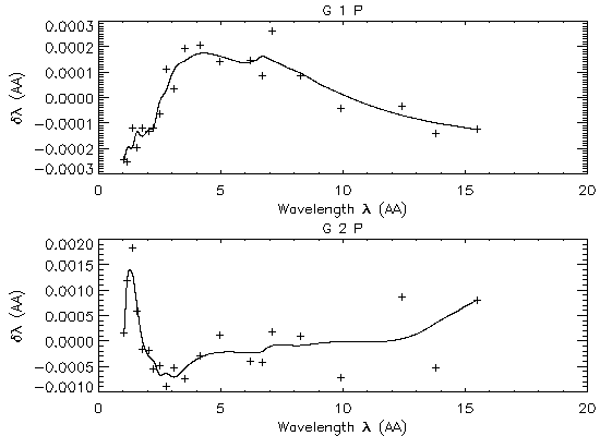
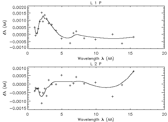
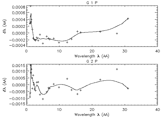
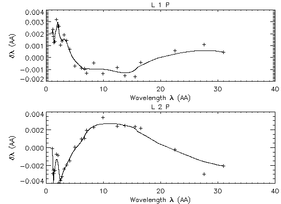
This step in the processing also minimizes any significant non-linearity in the wavelength/dispersion scale resulting from the instrumental design. Both HRC-S and ACIS-S, for example, form their detector surfaces by ajoining 3 to 6 planer-surface detectors (MCPs or CCDs), i.e., not precisely a Rowland torus (but mimicking closely by design). This type of non-linearity can be implicitly taken out with our new procedure.

Line Profile: Wavelength

Once again we run a number of mono-energetic marx simulations and analyze the line spectra by fitting a delta function with isis. The measured line centroid positions are then compared with the expected values to see the difference. Figures 9 and 10 illustrate the difference (Expected - Measured).

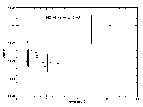
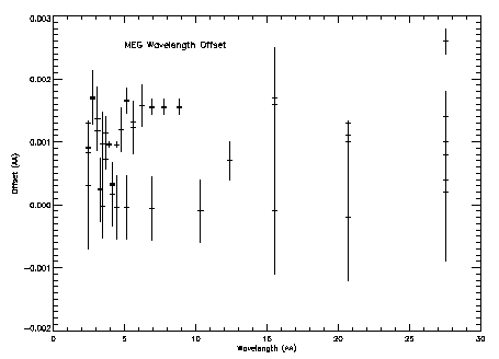
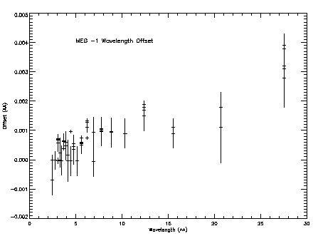
Figure 9: Wavelength offset (HEG): (top) HEG +1 order; (bottom) HEG -1 order.

Figure 10: The same as Figure 9 (for MEG +/-1 orders).

Note that the measured offsets are below the defined instrumental accuracy of HEG or MEG.

Addetum: J. Drake and D. P. Huenemoerder et al. inform me that the growing trend in offset seen in Figures 9 and 10 may be real and primarily due to some coding bug introduced within CIAO. The same effect is more noticeable in LETG/HRC-S (which would seriously affect users' scientific analysis with LETG/HRC-S).

Previous: Validation: Flux Estimate Next: Validation: Real HETG dataset

This page was last updated Dec 4, 2002 by Bish K. Ishibashi. To comment on it or the material presented here, send email to bish (at) space.mit.edu.