Introduction to crisscross: Extracting spectra from crowded regions¶

This notebook shows how to extract HETG spectra from a crowded region by running crisscross to handle confusion in two end-to-end examples:

1. covers a single ObsID in depth and
2. demonstrates how to run crisscross on multiple ObsIDs and combine the resulting spectra.

More information and examples on crisscross and its helper function clean_spec can be found on their respective ahelp pages (e.g., type "ahelp crisscross" and "ahelp clean_spec" on the command line in CIAO).

Crisscross Summary¶

crisscross and its helper tool clean_spec allow users to analyze Chandra High Energy Transmission Grating (HETG) spectra that are extracted from a field of view with multiple astrophysical X-ray sources. The HETG instrument will disperse events onto the ACIS CCDs from all sources in the field of view. If there are several sufficiently-bright X-ray sources then there is a potential for 'confusion' to occur. Confusion is a term used here for scenarios where standard HETG spectral extractions of a source may erroneously assign events (counts) from a different astrophysical source to the extracted spectrum. This can result in events from an unrelated astrophysical source 'confusing' the spectrum of an extracted source.

crisscross is used to identify when spectral confusion occurs for a list of input sources (or a single source) and generates 'confusion tables' which identify the wavelengths in each source's spectrum that are likely to include X-ray events from unrelated field astrophysical sources. The user can then choose to remove all events from the source spectrum in the wavelength range where this confusion occurs. The helper program clean_spec uses the crisscross output confusion tables and input HETG PHA spectra to generate 'cleaned' spectra (and ARFs) where these events are removed. crisscross is intended for crowded X-ray fields with multiple observations such as stellar clusters.

Running crisscross¶

First, packages and tools used later in the notebook have to be imported.

(1) Run crisscross for a single source on a single ObsID¶

This example uses ObsID 3, a crowded HETG observation of a pre-main sequence stellar cluster. The data is downloaded with the download_chandra_obsid script. A return value of "True" means that the download was successful.

The code below will extract the spectrum of a single source in the field of view using chandra_repro and the source coordinates. COUP 394 is a young, pre-main sequence star whose X-ray emission is generated by a hot corona. The commands below will produce only responses for the +1/-1 HEG/MEG orders. Users that wish to generate responses for more orders should use the 'tg_orders' parameter with chandra_repro.

Users that wish to see spectra from other sources in the field of view can modify the variables below before running the remaining cells.

Lets take a look at the source's spectra using Sherpa. We can use the sherpa-contrib function load_gratings_pha2 to identify and load the pipeline response files (ARFs and RMFs) whose names are in the PHA2 spectrum header. Since the PHA2 file contains all spectra for 12 orders (-3, -2, -1, +1, +2, +3 for HEG and MEG each), sherpa data ids 1-12 will be used. If the directory does not include all 12 HETG responses then only those identified will be loaded; this causes the warning messages below.

Now that the data are loaded, Sherpa can plot the brightest orders (HEG-1, HEG+1, MEG-1, MEG+1). Since there is not much data past 20 Å for this source, the plot limits the X-axis range.

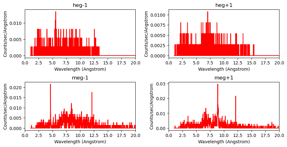
Similarly, the spectral response for the source can be plotted using the ARF files. This shows the sensitivity of the detector at the extracted spectral location.

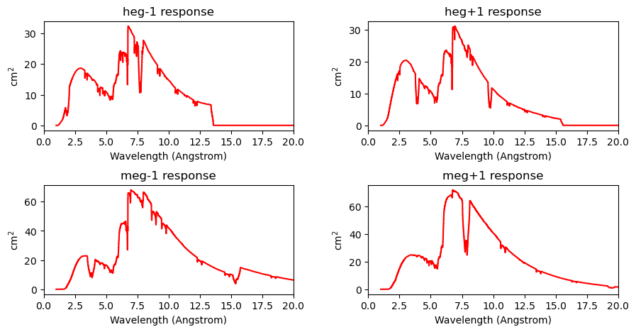
The event file can be viewed interactively with ds9. The following command will open ds9 in the separate window if this example is run on a local computer.

The extracted source is in a crowded field and confusion should be assessed. In other words, the dispersed spectrum of COUP 394 (green ds9 region-box if viewing the event file) intersects with many sources and other dispersed spectra. To identify potential confusion, crisscross will be run on the observation. This requires an input list of all X-ray sources potentially in the field of view.

Download source list for the tutorial: For this tutorial, a source list of X-ray sources in the field was prepared from Getman et al. (2005). To run this tutorial locally, https://cxc.cfa.harvard.edu/ciao/threads/crisscross/full_coup_src_list.tsv needs to be downloaded (e.g. right click and select "save as" on the link above) and saved in the same directory as the notebook.

For other fields, users will have to produce their own list of X-ray sources in the field that might cause confusion. Most of the Chandra HETG observations with more than a few sources in the field of view have been previously observed with Chandra imaging. Running CIAO's wavdetect on an archival non-HETG imaging observation is a good way to produce a source list. Otherwise, users will have to use another wavelength (telescope) or identify the 0th order sources in an HETG observation by eye and manually create a list.

An example of how to create a crisscross source list using wavdetect can be found on "ahelp crisscross".

The required inputs for this tutorial are a source list (which will be input to crisscross as the parameter main_list) and the evt2 file and RA/DEC of your HETG-extracted source. crisscross will identify if any of the sources in the source list produce erroneous counts in the extracted source COUP 394. Depending on the number of sources in the source list and the available hardware, crisscross could take a few minutes to run.

crisscross has now finished and produced the confusion table for COUP 394. dmlist (or any fits table reader) can show the identified confusion for each arm. Here, only the most relevant columns are selected for display.

crisscross identified some confusion (flag column 'confused'). The 'wave_low' and 'wave_high' columns indicate the wavelength range recommended to be ignored due to the likelihood of HETG confusion by source 'confuser_srcid'. The 'confusion_type' column shows which type of confusion (point source, spectral intersection, arm confusion, or read-out streak confusion) has been identified. For more information on each of these types of confusion, see "ahelp crisscross".

Next, the confused portions of the spectrum and responses are cleaned using the crisscross helper CIAO function clean_spec.

NOTE: clean_spec removes ALL counts in the confused regions and not just counts from the confusing source. However, crisscross has many tunable parameters to allow some level of potential confusion through based on the signal-to-noise ratio of the HETG source events compared to the confused events in the confused bandpass. If crisscross is unnecessarily removing counts it can be re-run with lower confusion threshold parameters. See "ahelp crisscross" for more info.

clean_spec will attempt to identify the relevant response files when provided with an HETG PHA2 file. This is important because clean_spec also zeros out the ARF for each region with confusion. The clean_spec tool creates a new 'cleaned' PHA2 file and associated ARFs and does not modify the original files. In this example, only 4 ARFs and spectra are cleaned because only 4 response files were created when running chandra_repro above (heg-1,+1, meg-1,+1). Even though only four orders have been cleaned, the new PHA2 file still contains the other 8 uncleaned (original) orders.

clean_spec produced a new PHA2 file and four new ARF files. They are loaded in Sherpa starting with ID 13 to avoid overwriting the previously loaded (uncleaned) spectra. load_gratings_pha2 will find the responses again and load the new cleaned ARFs and the original RMFs. RMF files do not have to be changed because of confusion and thus the same RMF files are used for original and cleaned spectra.

Now that cleaned spectra and responses have been prepared, a plot can compare the clean spectra to the original files that included confusion. This will demonstrate what crisscross and clean_spec have done.

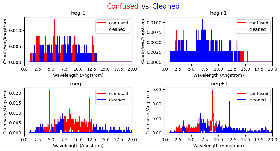
In the confused regions the flux (blue) is set to zero compared to the red spectra while in the other regions the blue and red spectra are identical (and the blue line is plotted on top of the red line). A similar comparison can be made between the original (confused) and cleaned arfs:

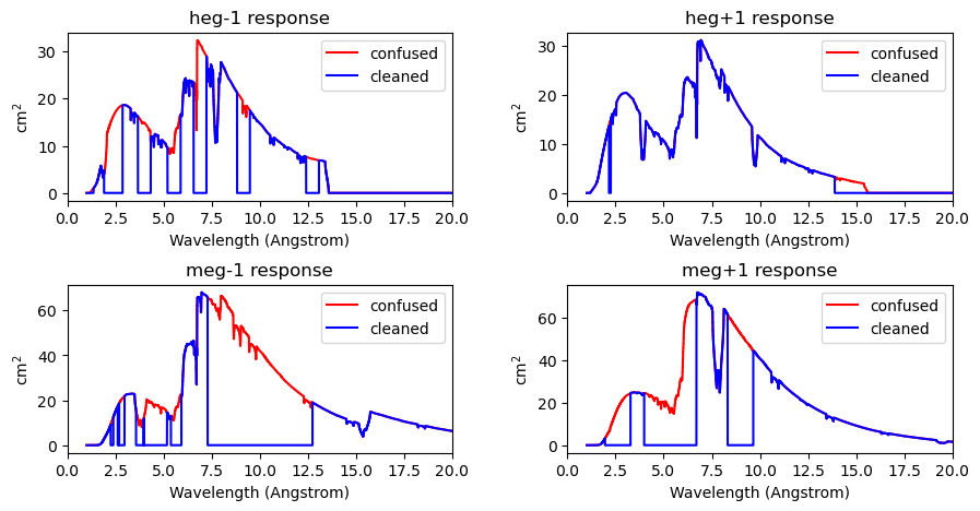
The plot shows that several portions of each spectrum have been identified to have events associated with other sources in the field assigned to the extracted COUP 394 source (i.e., confusion). What looked like an emission line at 8.5 Å in the meg+1 spectrum turns out to be emission from a different source crossing the extracted spectrum. The narrow ranges of confusion are typically associated with point sources or spectral intersection whereas the large bandpasses of confusion are typically the result of arm confusion (e.g., another bright source falling on the dispersed arm of the extract source.)

The confusion tables list specific instances of confusion and the source causing them. The code below lists confusion the MEG arm data.

From the table, it appears that the MEG+1 wavelength range of ~8-9.5 Å is affected by two sources of confusion. A 0th order point source (COUP 187) landed right on the dispersed spectrum and the dispersed spectrum of COUP 1390 also intersected with the extracted MEG+1 spectrum.

The events assigned to the HEG or MEG spectrum can be visually assessed to see how well crisscross identified confusion. This plotting method only works on evt2 files made for the extracted source of interest which in this case is COUP 394 since the grating coordiantes in the evt2 files are relative to that (a listing of the column names in the evt2 file is below).

The relevant HETG event values are copied to new arrays for plotting. HETG event files contain extra columns for events associated with the extracted spectrum compared to ACIS imaging observations.

This function filters the event file to retrieve order- and arm-specific event information for plotting.

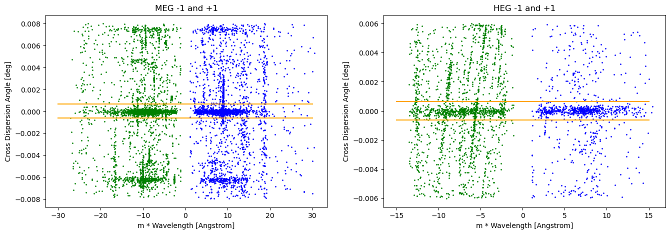
The above plot shows the MEG (left) and HEG (right) events associated with the CIAO extraction of COUP 394 source. Specifically, the events within the orange box will be those that are included in the PHA2 spectrum. The X-axis denotes the order * wavelength, so photons seen in a negative dispersion order are plotted at negative numbers. The y-axis denotes the cross dispersion angle (tg_d) in degrees, essentially the distance between a count and the middle of the line of dispersed photons.

A single unconfused source should only show events within the orange box. The MEG+1 plot (right, blue) shows a strong vertical line at about 9 Å which is the location of a 0th order (point source) field star that happened to fall on the dispersed spectrum of the extracted source. The vertical nature of this feature is due to the size of the PSF of that source. Many of those 0th-order events match the appropriate energy (e.g., 9 Å) to erroneously be assigned to the MEG+1 spectrum of COUP 394. Other fainter 0th-order confusing sources can be seen in MEG-1 at approximately -11 and -5 Å. The two large horizontal features shown in the MEG plot at y~0.008 and -0.006 represent the dispersed spectra of other stars in the field which are close to the extracted source. However, only events with a small range in cross dispersion angle (~+/- 6.3E-4) and assigned to the extracted source with CIAO tools.

The HEG -1 plot shows many examples of spectral-intersection confusion (e.g., the dispersed arm of another source overlapping the extracted source at the wavelength expected by ACIS order sorting). These are seens as with slanted lines at approximately -6.5 and -9 Å.

These plots can be hard to read when many sources are present, so the next plot filters out only the events within the orragne regions. For those events, the energy detected by the ACIS CCDs is then shown on the y-axis.

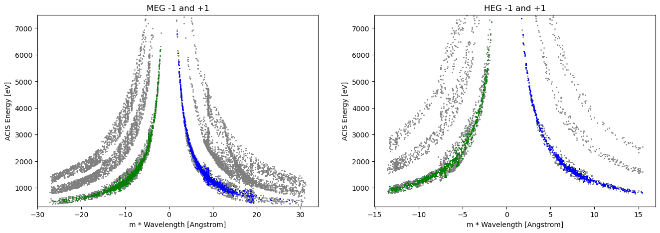
The above plots are the so-called HETG 'banana plots' and help reveal the extent to which a source's arm/order suffers from confusion. The HETG gratings equation determines the wavelength of every event based on its position along the dispersion direction from the 0th order. This wavelength (energy) is then compared to the ACIS CCD-determined energy of the same source to ensure it is compatible with the gratings-derived energy (wavelength). Only events whose ACIS CCD energy is consistent with the gratings-determined energy are ultimately assigned to the extracted spectrum with standard CIAO tools. Shown here in gray are all events assigned to any of the -3, -2, -1, +1, +2, +3 orders. The green and blue events are -1/+1 events that fall within the 4.6E-4 cross dispersion direction denoted by the yellow bars in the previous plots.

Looking closer at the MEG+1 portion of the spectrum one can see the previously discussed 'point source confusion' at ~9 Å. It shows us as a vertical bar in all three positive orders because the 0th order contains events at all energies and not just at 9 Å. Also note the curved feature starting at ~13 Å in the MEG+3 order (grey) and bending ultimately towards the MEG+1 order at ~ 20 Å. This is a clear indication of arm confusion from a source somewhere else on the detector but in line with the dispersed spectrum of our extracted source. The confusing source would likely contaminate all portions of the MEG+1 spectrum >~ 20 Å.

crisscross and its helper tool clean_spec facilitate the analysis of spectra from crowded HETG fields. The next and final step would be to fit the spectra with a model and learn something about the underlying astrophysics. This is beyond the scope of this tutorial but there are other CIAO tools that help with this process.

(2) Run crisscross for a single source on multiple ObsIDs and combine the spectra¶

Most HETG observations are campaigns with multiple ObsIDs. crisscross can process multiple observations and generate confusion tables for multiple sources in each ObsID. Users should see the crisscross and clean_spec help files for more examples of how this is done. The following example explains how to assess confusion for a single source over multiple ObsIDs.

First, download two more Orion Nebula Cluster pre-main sequence star observations and re-process them so chandra_repro extracts spectra of COUP 394.

Instead of running crisscross with a single evt2 file, here we will use a list of the three ObsIDs. They are identified with glob.

Crisscross output is saved to to a new directory.

To run clean_spec on multiple pha2 files the user needs to provide a list of pha2_files and the relevant crisscross confusion table files. Cleaned spectra are saved to a new directory.

Now there is a set of cleaned spectra from three ObsIDs, which will be combined with the CIAO tool combine_grating_spectra. This can be used for visualization purposes because it can combine multiple spectra of the same source from different obsIDs. It can also combine the +1 and -1 orders of the same arm. It should be noted that it is typically not best practice to fit combined spectra. Instead, users are encouraged to perform joint-fits on the individual spectra and use combined spectra for visualization purposes only. Moreover, caution should be taken when combining spectra from sources that undergo significant variability.

combine_grating_spectra looks for rmfs in the same directory structure as the PHA2 files so the original RMFs have to be copied to the new 'cleaned' directory to combine all the cleaned files and responses. This is usually managable but RMFs can be relatively large files, so soft links or other ways to minimize disk usage might be useful.

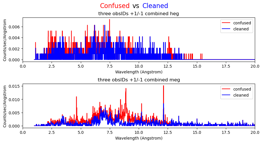
The code below loads the COUP 394 spectra combined from three ObsIDs into sherpa and plots the comparison of the confused vs cleaned spectra again.

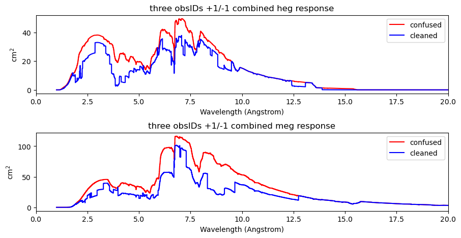
As exposure time is increased with multiple ObsIDs, more emission lines are visible for COUP 394. Also note how the combined response does not go to zero because confusion does not occur at the same spot in all ObsIDs due to roll angle variations and source variability. Multiple observations can be used to mitigate confusion in crowded regions.This comparison of the original (confused) data with the cleaned data demonstrate the necessity to account for confusion from other sources in the field of view.

This also demonstrates how cleaning spectra takes away signal, which includes real data, too. In the MEG there is significant emission in the (real) Ne X emission line at 12.14 Å. However, in one of the observations a large region of the arm is potentially confused as thus filtered out (see the lower panel in the ARF plots, where the "cleaned" ARF is significantly below the "confused" ARF below 15.7 Å). This confusion is relevant for large ranges of that spectrum, in particular in regions where the source is weak. However, at 12.14 Å the source is so strong that is outshines any confusion, yet the real counts are also removed when the entire region is masked as "potentially confused" by crisscross. In that sense, crisscross is desined to be conservative and to mask all regions with potential confusion, but it is possible that this also removes counts in areas where the source is so bright that the relative contribution of the confusion is not significant.

For questions, comments or suggestions about crisscross and its functionality, please contact the CXC helpdesk or through email at cxchelp@cfa.harvard.edu.