Guide to using srcflux for acis_extract users
Introduction
This guide discusses the basic differences between CIAO's srcflux tool and ACIS Extract. It is not meant to be an exhaustive comparison of all the capabilities, algorithms, and outputs of each tool, but rather is meant to be a quick guide for acis_extract users who want to use srcflux.
Both tools produce estimates of a source's count rate and estimates the flux with uncertainties. As part of this processing they produce several data products for which users may find additional uses. Under the hood, acis_extract uses the same CIAO tools as srcflux along with a few tools from HEASOFT/FTOOLs package. Therefore it is unsurprising that the results from the two tools are consistent.
Relevant threads:
Summary
Here is a quick summary of the key features of both srcflux and acis_extract.
| Feature | srcflux | acis_extract |
|---|---|---|
| Refine source position (multiple options) | (1) | ✓ |
| Compute source significance (SNR) | ✓ | ✓ |
| Adjust regions for crowded fields | ✓ | ✓ |
| Extract source and background spectra | ✓ | ✓ |
| Adjust ARF for energy dependent PSF fraction | ✓ | ✓ |
| Extract lightcurves and provide variability metrics | ✓ | ✓ |
| Photometry | ✓ | ✓ |
| Spectral modeling | (1) | ✓ |
| Collates results | ✓ | ✓ |
| Visual Review | ✓ | |
| Combine multiple observations | ✓ | ✓ |
| Diffuse sources | ✓ | ✓ |
| XMM EPIC | ✓ | |
| HRC | ✓ | |
| PIMMS-like fluxes | ✓ |
- srcflux does not provide this type of analysis. However, it has been upgraded to allow users to run arbitrary custom analysis scripts, "plugins", and include the results in the output *.flux file. Users can write and run plugins to fit spectra and compute new source positions or any additional analysis they wish to perform (compute hardness ratios, radial profiles, period folding, etc.)
These are just the key features of both tools. They each produce additional outputs that are considered to be diagnostic or informative rather than essential outputs.
Basic differences
Comparing interface
|
srcflux is a python script that runs like any other CIAO tool either from the command line or in python via the runtool module. Everything needed to run srcflux is provided with CIAO, with the optional installation of MARX. |
acis_extract is written in the language of the commercial product IDL; licensing, availability, and costs of IDL are beyond the scope of this guide. acis_extract also requires CIAO, MARX, FTOOLs, and third party IDL packages (astronomy package and its dependencies). |
|
The key inputs to both tools are the input event file(s) along with the celestial coordinates of the source(s) to analyze. Both tools will, with proper setup, be able to locate the auxiliary files needed for data analysis (aspect solution, bad pixels, and mask files); alternatively, both tools will allow the user to specify the location of these files explicitly. |
The only key difference here is that acis_extract requires an input exposure map and set of aspect histograms files (and it provides a helper script to generate these); whereas srcflux creates these files as needed. |
|
Both tools produce text output to the terminal with the analysis results as well as saving the results to FITS tables. srcflux does not produce tables in LaTeX format; however, the srcflux output .flux file can be displayed directly in ds9 as either a region file or as a catalog: $ ds9 acis_evt2.fits -region out_broad.flux -or- $ ds9 acis_evt2.fits -catalog import fits out_broad.flux |
acis_extract also provides some ds9 displays for the source positions along with a helper script to convert the output into a LaTeX format table. |
|
By default srcflux runs most of the analysis commands in parallel taking advantage of all CPUs. |
acis_extract runs commands serially, but has recipes for running multiple OBS_IDs in parallel. |
Difference in default extraction regions
Both srcflux and acis_extract allow users to supply their own source and background regions; eg ds9 format region files. However, both provide default regions, which have some differences. For most sources there will be no significant difference in flux estimates which have been corrected for exposure and PSF fraction; the most significant differences will be seen in very dense, crowded fields.
|
The default source region for srcflux is a circular region that encloses approximately 90% of the PSF at 1.0keV. The radius is derived from the PSF REEF calibration data product which was derived for a flat detector such as ACIS-7 and HRC. While it is less accurate for other chips, the actual PSF fraction is computed separately from MARX simulates (with psfmethod=marx). The default background region is an annulus whose inner radius is equal to the source region radius, and whose outer radius is equal to five times the source region radius. Nearby sources are excluded from both the source and background region. |
The default source region for acis_extract is a polygon that encloses 90% of the PSF at 1.49keV. acis_extract uses MARX to simulate the PSF at the source location, smooths it, and finds a contour that encloses 90% of the PSF. Given the shape of the PSF, increasing the size of the extraction region can actually result in a decrease of the SNR; the acis_extract polygon regions therefore try to optimize the region for true point sources. Since these are derived from simulations there is a degree of randomness in the results. Generally these polygons are nearly elliptical with small scale perturbations. However, note that the actual polygon is only used to create a mask so randomizations and perturbations smaller than a pixel do not matter. For the background regions, acis_extract has an iterative procedure to create an annulus around the source and increase the outer radius until it has achieved a certain threshold (eg number of counts) -- while excluding nearby sources. For nearby sources, the source region is shrunk by reducing the fraction of the PSF of the neighboring regions until they no longer overlap. This has the same net effect as the srcflux approach of simply ignoring pixels, but the srcflux only ignores pixels in the overlap region, whereas the smaller polygons exclude pixels on all sides of the source. This makes sense for acis_extract since it also can refine the source position and having an asymmetric region would bias the results. |
Differences in default energy bands
Both srcflux and acis_extract allow users to analyze multiple energy bands.
|
The srcflux default energy band for ACIS is 0.5 to 7.0keV matching the broad energy band used in the Chandra Source Catalog. Users can specify the acis_extract bands using the following parameter setting $ pset srcflux bands="0.5:2.0:1.49,2.0:8.0:3.0,0.5:8.0:2.3" The 3 colon separated values represent the minimum energy, maximum energy, and the characteristic energy used to create the exposure maps and PSFs. |
acis_extract by default produces results for several energy bands. When the final collate_results step is run though, only 3 bands are left: s (soft), h (hard), and t (total). The soft band goes from 0.5 to 2.0keV, hard band goes from 2.0 to 8.0keV, and the total band goes from 0.5 to 8.0 keV. |
Since the ACIS effective area is very low between 7.0 and 8.0 keV, we can safely directly compare the srcflux default broad with the acis_extract total band.
Matching data products
Below is a table showing the mapping of the important data products created by both tools, with some notes about key differences.
| Data Product | srcflux (1) | acis_extract (2) | Notes |
|---|---|---|---|
| Exposure Map files | *_thresh.expmap | background.emap source.emap |
(3), (4) |
| Event files | background.evt neighborhood.evt source.evt |
||
| Images | *_thresh.img *_flux.img |
||
| Region files | ${outroot}_${id}_bkgreg.fits ${outroot}_${id}_reg.fits ${outroot}_${id}_srcreg.fits |
extract.reg | (6) |
| Spectra | ${outroot}_${id}.pi ${outroot}_${id}_bkg.pi |
background.pi source.pi |
(5) |
| ARF files | ${outroot}_${id}.arf ${outroot}_${id}_nopsf.arf ${outroot}_${id}_bkg.arf |
source.arf source7.arf |
(7), (8), (9) |
| RMF files | ${outroot}_${id}.rmf ${outroot}_${id}_bkg.rmf |
source.rmf | (7) |
| PSF files | *.psf *_projrays.fits |
source.psf obs.psffrac |
|
| Lightcurve | *.lc *.gllc |
source.lc | (10), (11), (12), (13) |
| Source Properties | ${outroot}_${band}.flux ${outroot}_summary.txt |
obs.parameters obs.stats |
- The srcflux files are prefixed with ${outroot}_${id}_${band}_, where ${outroot} is the user supplied output filename root, ${id} is the source number going from 1 to the number of sources (same as the COMPONENT value in the output .flux file), and ${band} is the band name or energy limits if not one of the CSC named bands.
- All acis_extract files are stored in a sub directory ${coordinates}/${obsid}, where ${coordinates} is the sexagesimal representation of the input RA and Dec and ${obsid} is the OBS_ID of the observation.
- srcflux creates a single exposure map that encloses both the source and background regions, whereas acis_extract creates individual cutouts from the input exposure map around the source and background regions separately.
- srcflux creates the exposuremap at the characteristic energy for each energy band, whereas acis_extract uses the single exposure map provided by the user for all bands.
- srcflux uses the CIAO definition of BACKSCAL: which is the ratio of the geometric area of the extraction region to the total field area. acis_extract uses a different definition of BACKSCAL related to the sum of the exposure map pixels in the extraction region.
- The acis_extract extract.reg file has both the source polygon and the background circle
- By default acis_extract does not produce background response files (ARF and RMF). srcflux does created these files by default, but they can also be skipped.
- srcflux uses mkwarf to create weighted response file (even for on-axis sources). acis_extract uses mkarf to create point-like responses (even for off-axis sources)
- srcflux adjusts the effective area for the fraction of the PSF in the source region using the arfcorr tool, which uses the REEF circular approximations to the PSF. acis_extract simulates the PSF at multiple energies and corrects the effective area by interpolating the PSF fraction it derives at those energies.
- The acis_extract light curve is for the total energy band. The srcflux light curves are for each individual energy band.
- The acis_extract light curve contains the total source region count rate. Each srcflux light curve has separate source, background, and net count rates.
- The acis_extract lightcurve also contains grouping information (ie to produce bins with a minimum number of counts). It also contains the median energy of the events during the time bin.
- srcflux also creates the adaptively binned lightcurve created using the Gregory-Loredo algorithm to check for variability and reports a variability probability. acis_extract computes a variability probability using a KS test.
There are also other additional diagnostic and intermediate files created by each tool.
Matching source properties
Both tools produce source properties for a each individual observation, and for the merged/combined dataset.
Per Observations Properties
All of the srcflux source properties are stored in the output .flux file. There are nearly 60 columns, the details of which can be found in the srcflux help file. To briefly summarize, it outputs
- Coordinates: celestial, sky (physical), chip, off-axis angle
- Region information: shape, radii, rotation angle, area, mean-exposure
- Validity flags: near chip edge, inside field-of-view
- PSF information: psf fraction
- Photometry: counts, net-counts, rates, photon fluxes, model-independent fluxes, PIMMS-like absorbed & unabsorbed model fluxes.
- Variability: G-L probability and odds
The acis_extract source properties are stored in several different files including the obs.parameters, obs.stats, source.stats, source.photometry, and the ObsIDs_merged.fits files. Collectively these outputs have much of the same information as srcflux which sufficiently similar column names that the mapping is obvious. Some less obvious mappings and differences include:
- In the source.photometry file, the FLUX1 values are similar to the srcflux model-independent NET_FLUX_APER fluxes. The FLUX2 values are equivalent to the NET_PHOTFLUX_APER photon fluxes.
- acis_extract computes several energy percentiles (25%, median, 75%) which srcflux does not compute.
- In addition to a source significance computed by both tools, acis_extract also computes a probability of not being a source, PROB_NO_SOURCE
Properties for combined datasets
The srcflux merged results are also stored in a single .flux file. It contains a subset of the source properties which includes things like the combined rates and fluxes.
The acis_extract values are combined during the collate step and are written to the output xray_properties.fits file.
The most meaningful common property is the photon flux values, since things like differences in regions/areas/psf-fractions will all be accounted. srcflux computes two estimates of the photon flux: MERGED_NET_APRATES_PHOTFLUX_APER and MERGED_NET_PHOTFLUX_APER. The former is derived by running the aprates with essentially exposure and psffraction weighted per-obsid properties. The later is simply the combined counts divided by the combined exposure map. The broad band MERGED_NET_PHOTFLUX_APER value then most closely matches the acis_extract PhotonFlux_t value; the acis_extract collate step renames FLUX2 to PhotonFlux.
Note that the acis_extract EnergyFlux is not equivalent to the srcflux eff2evt NET_FLUX_APER or TOTAL_FLUX_APER. As per the comments, the EnergyFlux is simply the PhotonFlux scaled by the median energy. (It is not the same as the FLUX1 values.)
Comparing Results
We now show some comparisons of running srcflux and acis_extract.
For srcflux we used psfmethod=marx and set the confidence limit to 68% (conf=0.68). To save time we also skipped creating background response files, ie bkgresp=no.
For acis_extract we followed the thread shown in section 3, Getting Started, of the acis_extract users guide, with the additional step of running ae_flatten_collation to provide the simplified final output xray_properties.fits file.
The best value to compare is the photon flux values (photon/cm^2/sec) since it is has all the corrections for exposure and aperture area/PSF fraction.
Comparing results for a single observation
For our single obsid test case we used OBS_ID 4396, a 170ksec observation of the Orion field. For our source positions, we queried version 2.0 of the Chandra Source Catalog and used the location of the sources in the field of view for this obsid. There are 1440 source locations. The srcflux command line looks like
$ srcflux acisf04395_repro_evt2.fits pos=csc.fits bkgresp=no psfmethod=marx conf=0.68 clob+
Below is plot showing a comparison of the Photon flux values from srcflux on the X-axis vs. acis_extract on the Y-axis. The solid diagonal line is 1:1. The symbols are color coded by the TOTAL_COUNTS in the source region as reported by srcflux. The text label is the source number, COMPONENT value, in the source flux output.
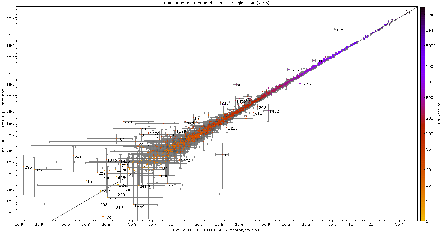
Overall we see excellent agreement between srcflux and acis_extract especially for sources with more than 10 counts. Below 10 counts there is more scatter, but the given the uncertainties the agreement is good. As one might expect there are a few outliers. We have identified two for closer inspection.
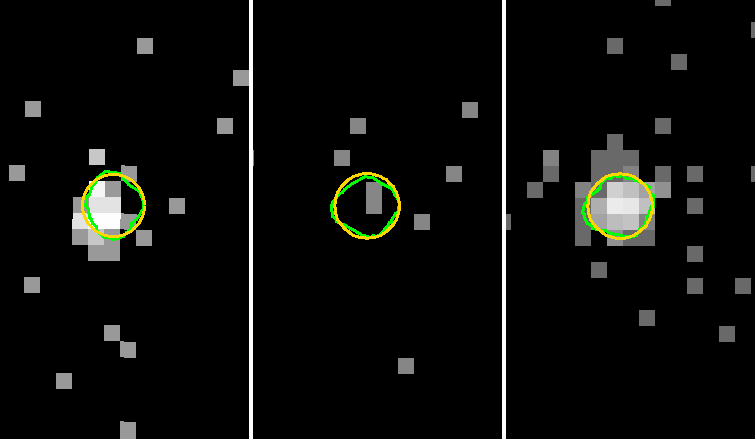
Region 105
Region 105, on the upper right quadrant of the plot, shows a significantly higher photon flux estimate from acis_extract compared to srcflux. It has a relatively large number of counts so we would expect better agreement. The regions used by srcflux and acis_extract are shown below:
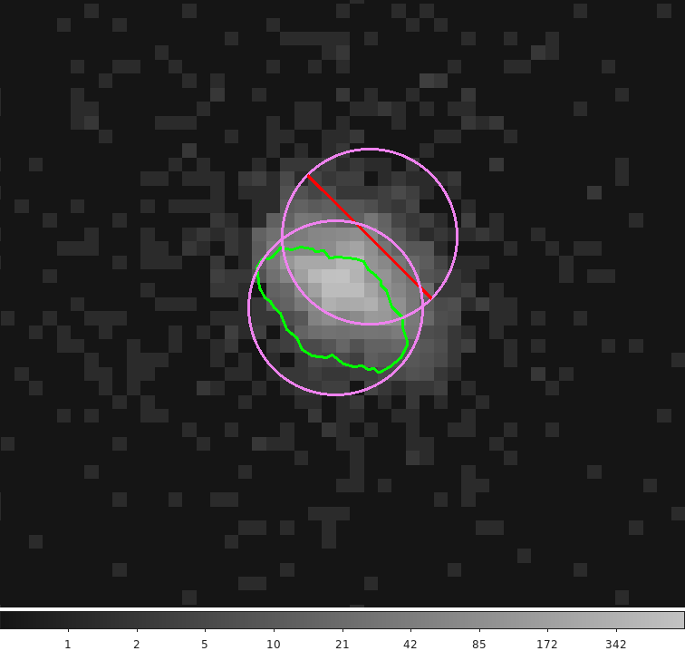
From this we see that there were two nearby sources identified in version 2.0 of the Chandra Source Catalog. (Why? Remember that the CSC is obtained by detecting sources in merged datasets. It is probably the case that what looks like one off-axis source is resolved into two nearby source when imaged on-axis.) The purple circles are the srcflux regions; where the northern source is excluded from the southern source, leaving a crescent moon shaped region. The center of the source is offset from the peak emission which is excluded by the neighboring source. The green polygon is the acis_extract region, which even though is offset from the source center, does include the peak emission. This is why the acis_extract photon flux estimate for this source is higher than the srcflux value. It is not entirely clear here how acis_extract is handling these crowded sources. The manual discusses an algorithm to shrink the source regions when they overlap. It is unclear whether the way we ran acis_extract in this example will trigger this algorithm.
This is a good example of why it is important to properly vet the input source catalog/source list. In this example we would argue that this is a poor choice for source locations and as such neither tool will produce robust results.
Region 816
This regions is located center of the plot, below the 1:1 axis. In this case, the srcflux photon flux is an order of magnitude higher than the acis_extract estimate (1.5E-6 vs 1.4E-7). The regions are shown below:
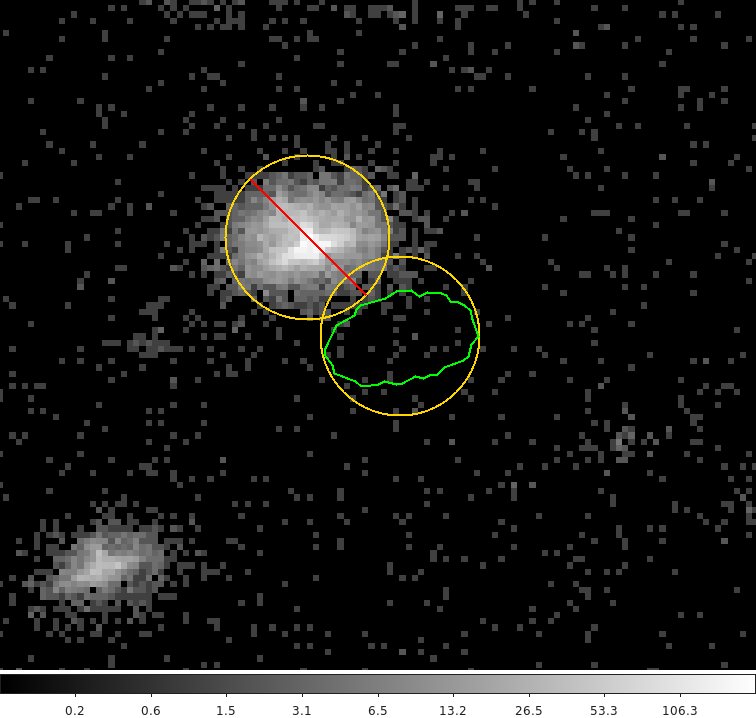
Again this is a case of two nearby, overlapping source regions. In this case a very bright source is nearby this very faint source. The srcflux regions are the yellow circles showing the bright source being excluded from the faint source. The green polygon is the acis_extract region. In this case the acis_extract region does happen to be a better aperture choice. While srcflux is excluding most of the bright source from the faint source, we do see some of the wings of the PSF from the bright source showing up in the faint source's region. This is artificially increasing the flux estimate of the faint source compared to the regions acis_extract is using.
Comparing results for a merged dataset
For a second comparison we show the results comparing srcflux and acis_extract for a merged dataset. For this example we chose the 3 observations of the Open Cluster Collinder 197
| OBS_ID | DATE-OBS | Exposure (ksec) |
|---|---|---|
| 22689 | 2021-01-01 23:55:24 | 34.62 |
| 25099 | 2021-07-30 06:13:40 | 11.0 |
| 24757 | 2021-08-17 06:33:01 | 24.94 |
The data were reprocessed with chandra_repro, and combined with merge_obs. We then ran wavdetct on the combined image and detect 258 sources. When ran srcflux and acis_extract with the same setup and parameters as for the single observation test.
Below is a plot comparing the broad band photon flux values
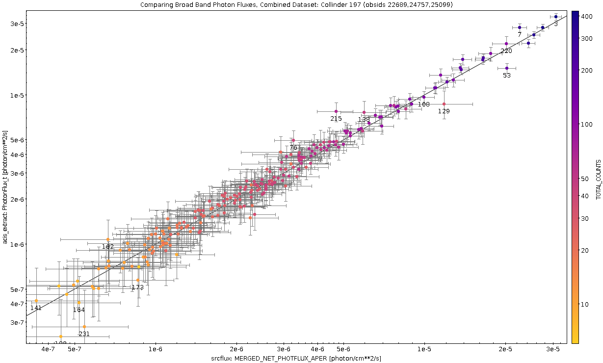
As before, the X-coordinates are the srcflux photon flux estimates and the Y-coordinates are the acis_extract photon flux estimates. The srcflux values are the MERGED_NET_PHOTFLUX_APER values taken from the combined .flux file, the acis_extract values are the PhotonFlux_t values from the collated xray_properties.fits file. The diagonal line is 1:1 (two values are equal). The points are color coded by the srcflux TOTAL_COUNTS, and the number labels are the srcflux source ID number.
There are a few outliers that are worth examining, although the discrepancies are not as significant as in the single observation example.
Region 53
Region 53 is one of the brightest sources. The srcflux photon flux estimate is somewhat higher than the acis_extract estimate. The per-observation apertures are shown below
The images are for the observations in left-to-right order of observation date: OBSID 22689, 25099, 24757. The srcflux circles are in yellow and the acis_extract polygon are green. The regions are nearly identical for this nearly on-axis source. However, when we look at the fluxes for each individual observation
| OBS_ID | Photon Flux (ph/cm**2/sec) |
|---|---|
| 22689 | 3.36E-06 ( -0.68E-06,+0.77E-06 ) |
| 25099 | 9.04E-07 ( -5.56E-06,+9.06E-6 ) |
| 24757 | 5.22E-05 ( +/-0.43E-05 ) |
the source is variable. In this case a single combined flux estimate is not meaningful. The difference then may arise in how variable sources are treated. Users would need to be cautious when publishing this source's properties.
Region 215
The acis_extract photon flux estimate for region 215 is higher than the srcflux estimate (located near the center of plot). Again we start by examining the source regions
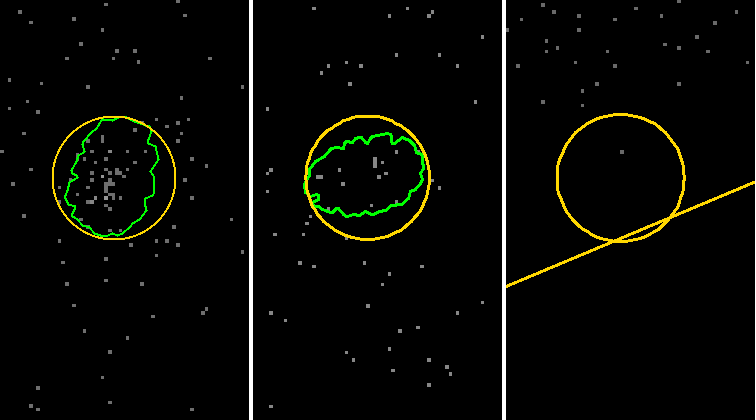
The per-observation images are in left-to-right date order. The yellow regions are the srcflux circles and the green polygons are the acis_extract apertures. The source is located at the edge of the field of view for obsid 24757 (the line segment in the right image is part of the FOV boundary). In this case, acis_extract did not produce any results for this observation (not even a region) whereas srcflux used the available one count to produce an upper limit. The upper limit in this case is slightly pulling down the overall mean value from the other two which is the reason for the difference between the acis_extract and srcflux results.
Conclusions
This guide provides information that users familiar with acis_extract may find helpful when using the srcflux tool. It is far from an exhaustive comparison of the features of each tool, but instead focuses on the results obtained with the default settings. Both tools produce a cache of useful data products for individual sources in separate observations as well as combined/merged products for sets of observations. While there are subtle differences in how the two tools work, the end results are shown to be in excellent agreement. The outliers have been shown to be a consequence of the different default aperture algorithms or due to exceptional characteristics of the data.