Mission Planning Update
Scott Randall, Daniel Castro, Tara Dowd, Ewan O’Sullivan, Joshua Robbins, Iris Wang, and Joshua Wing
It has been many years since the Mission Planning Team has directly contributed to the Chandra News. During that time, there have been a number of significant updates to the procedures, tools, and software that the team uses to address new scheduling challenges as they arise. This article will summarize some of the main scheduling issues and highlight just a few of the most important updates that have been implemented to address them.
Thermal Balance

Figure 1: The thermal behavior of various Chandra subsystems as a function of solar pitch angle. For each subsystem, blue indicates that at that pitch angle the subsystem will be moving away from the limiting temperature, gray indicates no significant temperature change (neutral), and pink indicates the subsystem is moving towards the limiting temperature. Dark red indicates that at that pitch angle the given subsystem is the one that most tightly limits the maximum dwell time. There are no pitch angles at which the dwell time is not limited by some subsystem.
The main goal of Mission Planning can be stated simply: to maximize the science return of the mission in the presence of constraints while ensuring the health and safety of the spacecraft. These constraints can be roughly divided into two classes: science constraints defined by observers to ensure that the science goals can be met (e.g., coordination constraints, observing window constraints, roll angle constraints) and operational constraints that ensure the quality of the science data as well as the health and safety of the spacecraft (e.g., bright source avoidance, subsystem temperature limits, reaction wheel momentum limits). Here, we will focus on operational constraints and their evolution over the years as well as how the Mission Planning Team has managed these issues.
Currently, the main issue driving Chandra's scheduling complexity is the need to stay within the temperature limits of the various subsystems. This was not a significant issue earlier in the mission; however, the ongoing degradation of the multi-layer thermal insulation has resulted in a significant increase in the mean temperature of the spacecraft. The current state of affairs is summarized in Figure 1. Since each subsystem is located on a distinct part of the satellite, they generally heat and cool differently as a function of the spacecraft's pitch angle relative to the Sun. The dark red bands in Figure 1 indicate that, over the indicated pitch range, the corresponding subsystem limits the amount of time that Chandra can dwell at that pitch. Once that limit is reached, the spacecraft must go to a pitch range where the subsystem in question cools (indicated by the blue bands) before going back to a heating pitch angle. An important point is that there is no pitch angle where the dwell time is not limited by the temperature of one subsystem or another—i.e., there is no pitch angle at which all subsystems cool and Chandra can therefore dwell indefinitely (at least not without powering down subsystems that are essential for observing). Thus, modern-day scheduling is largely based on carefully maintaining a delicate balance between subsystem heating and cooling.
The Chandra-Spike Assistive Scheduling Software
The thermal limitations described above lead to an immediate scheduling issue. For a collection of targets (e.g., those to be observed in a given week), observations that heat a particular subsystem must be paired with observations that will cool that subsystem down to at least the starting temperature. Some subsystems heat and cool similarly as a function of solar pitch angle, as can be seen in Figure 1, and can therefore be combined into one "thermal group" that guides scheduling. We require a minimum of 5 such thermal groups to adequately control subsystem temperatures. This means that when laying out the year-long Long Term Schedule (LTS), hundreds of observations have to be placed into 52 weekly bins such that each of the 5 thermal groups is balanced, keeping in mind that the solar pitch angle of each target changes throughout the year. Simultaneously, other scheduling restrictions must be met. For example, higher operating temperatures for the aspect camera assembly (ACA) mean a higher detection threshold for the stars used to determine the pointing. As a result, sparse star fields must be done on certain days of the year when the roll angle is favorable and sometimes at lower than usual ACA temperatures. In addition to LTS bins that are thermally balanced, targets must be grouped to give a momentum balance, such that the reaction wheels can be used to manage momentum, thereby minimizing the number of thruster firings for momentum unloading. The sky distribution of targets must also be balanced in each bin, according to a metric that we have defined, to optimize maneuvering between targets. Finally, the science scheduling constraints that are defined by observers must also be satisfied.
Building a year-long schedule that satisfies all of the above requirements is a mathematically complicated problem. Out of all the possible LTSs that can be constructed by randomly dropping targets into weeks, only a very small fraction of them are thermally balanced for every week. Finding these schedule "solutions" is extremely challenging, and due to the scale of the problem a brute force approach is not feasible. One of the main achievements of mission planning over the past several years has been the development of the Chandra-Spike assistive scheduling software to help address this issue. Developed in collaboration with a software engineering team at STScI, Chandra-Spike uses a genetic algorithm to generate tens of thousands of possible schedules, each scored using a set of pre-defined metrics. The specialized input format is extremely flexible, abstracting the problem into the concept of various "resources" (including the time available per week and the "thermal budget" available for each thermal group) that are impacted by "actors" in each bin. Actors (observations) can both provide additional resources (e.g., cooling) and consume resources (e.g., heating), and the combination of actors in a bin gives the total resource balance. The impact of actors on resources in future bins is estimated from detailed models of the spacecraft and subsystem behavior. These predictive models are frequently updated based on comparisons with the actual measured subsystem temperatures on the spacecraft. This flexible design has proved invaluable for scheduling, as it allows new resources to be defined as different subsystems and other constraints come into play.
In practice, when used to construct the LTS, Chandra-Spike produces some number of acceptable schedules, which Mission Planning then scores using a set of posterior metrics to choose the best "starting point LTS." Manual adjustments are still needed before a final schedule is ready for implementation, but Chandra-Spike has nevertheless been hugely successful, reducing the time taken to construct the LTS from several months when done "by hand" to a few weeks. As the complexity of the problem has only increased with time, it is safe to say that the construction of a highly efficient and thermally balanced LTS would no longer be possible by hand.
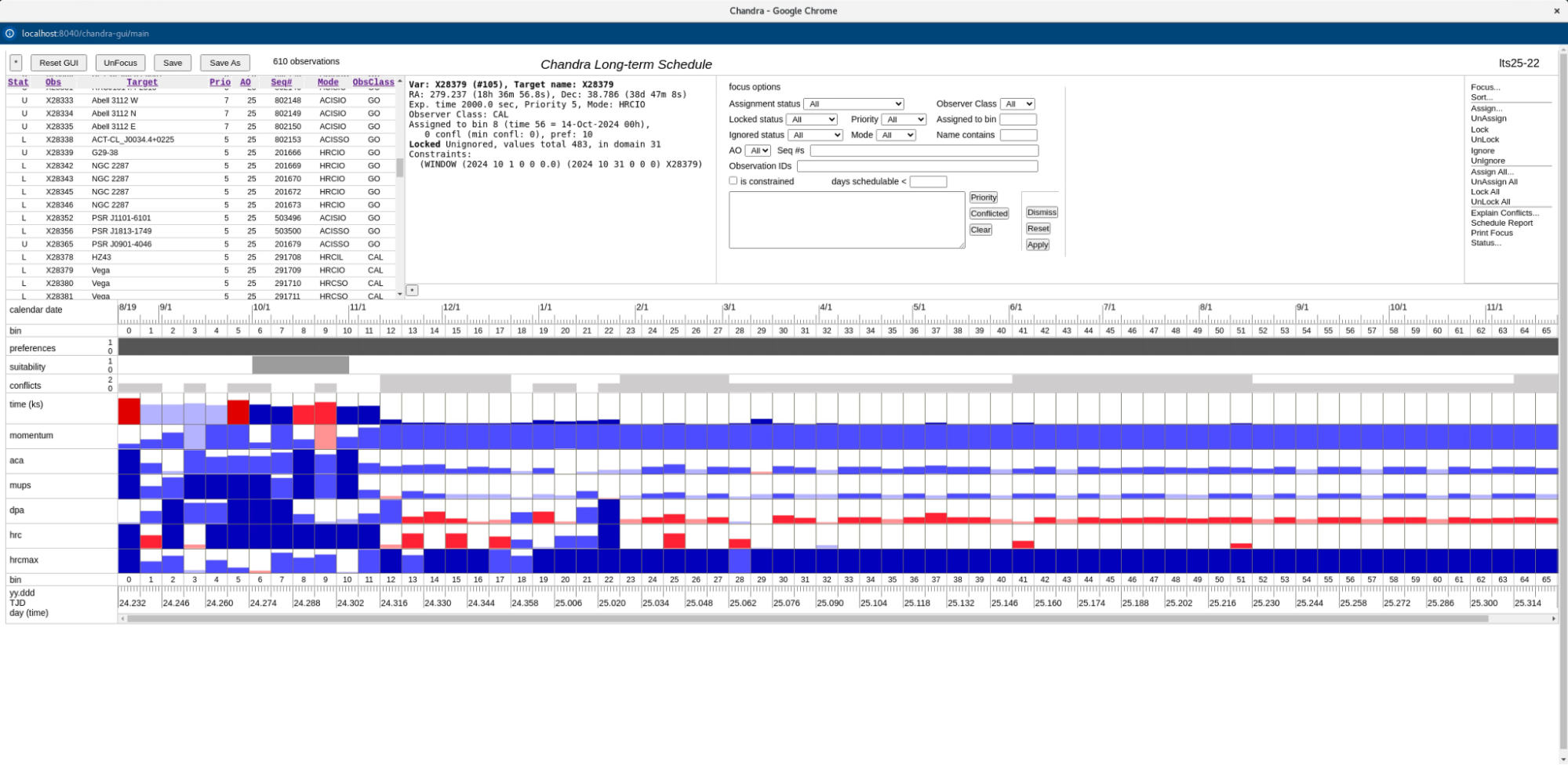
Figure 2: A screenshot of the front-end GUI to Chandra-Spike, used for checking and performing minor adjustments to the LTS during weekly scheduling. The timeline indicates the usage of the various resources, color-coded from dark red (overused) to dark blue (remaining resources).
Over the past year, we finished developing and fully implemented a front-end GUI to Chandra-Spike. This tool is used weekly to perform maintenance on the LTS, which is needed as the schedule changes to accommodate targets of opportunity (ToOs), shutdowns due to solar flares, and other similar unforeseen events. A screenshot of this GUI is shown in Figure 2. When an observation is selected from the list in the upper left corner, the impact it would have on the various resources and other metrics if scheduled in a given week is immediately shown for each bin in the color-coded timeline. Having this information readily accessible greatly simplifies the process of deciding where any new or rescheduled observations should be placed in the LTS.
Resource Cost
Another key advancement in mission planning over the past several years has been the development and implementation of the concept of a Resource Cost (RC) for a given observation. Prior to Cycle 22, constrained observations were grouped into one of three broad constraint categories: Easy, Medium, or Difficult. As the complexity of scheduling grew with time, it became clear that these categories were insufficient to capture the full range of "burden" associated with proposed programs. Furthermore, the thermal limit issues described above mean that the difficulty associated with scheduling observations needs to be tracked even for observations with no science constraints. The concept of a Resource Cost reduces the burden of any given observation to a single number. This number is derived from a series of empirical models associated with various science constraints and by the pitch distribution and visibility of the target throughout the observing cycle. Thus, the impact of thermal limitations is naturally folded into the total RC. At peer review, there is a total RC budget that is not to be exceeded by the combined RC of all recommended observations. This ensures that the yearly accepted target list can be efficiently scheduled (in principle) during the relevant observing cycle. Observers can use the public-facing version of the Resource Cost Calculator Tool to calculate the RC of any hypothetical observation before submitting an observing proposal. The Resource Cost distribution for all accepted non-ToO GO programs from Cycle 14 through Cycle 27 is shown in Figure 3.
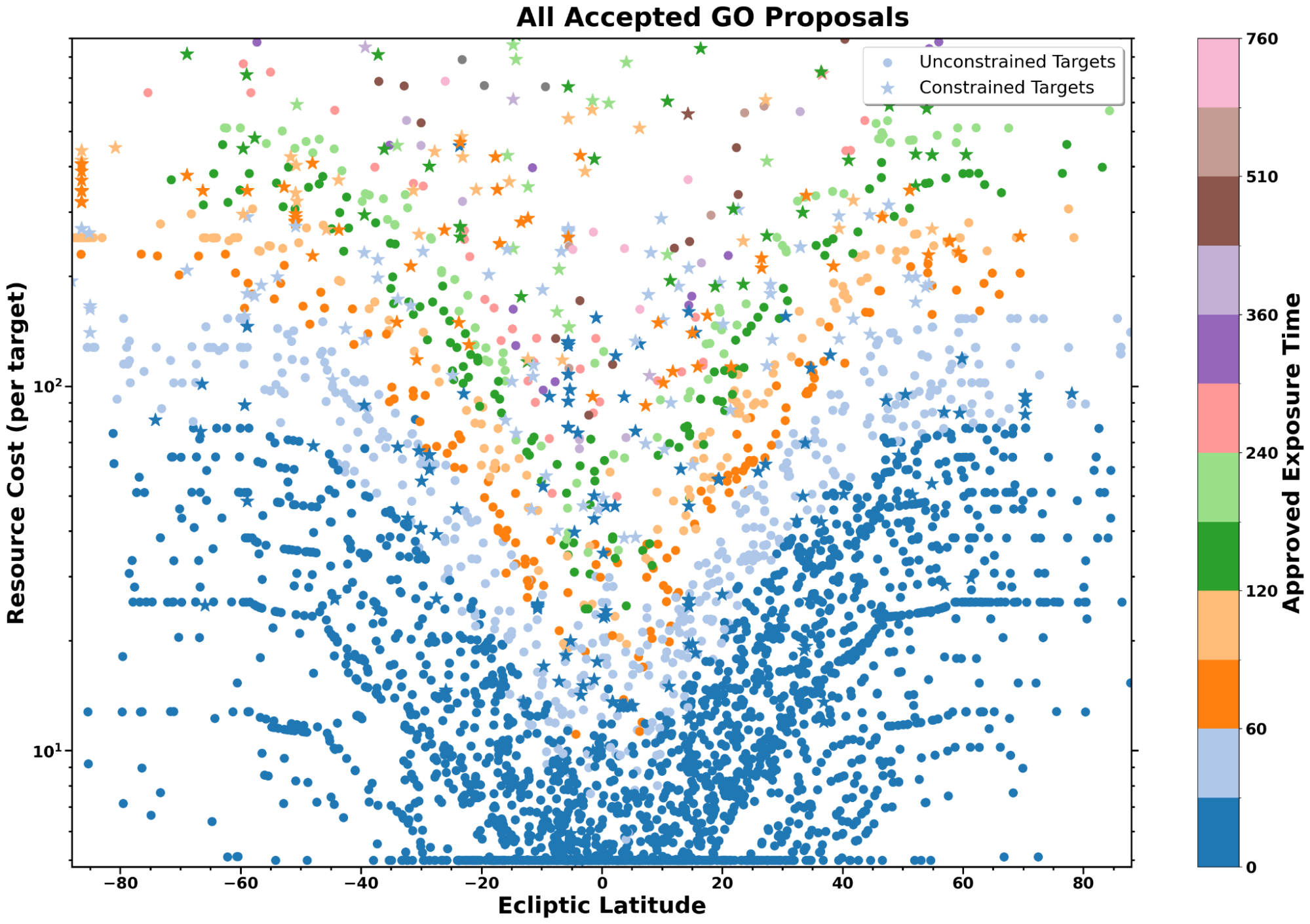
Figure 3: Resource Cost values for accepted observing programs from Chandra Cycles 14–27, color-coded by the approved exposure time. Starred targets have science observing constraints, circles are unconstrained.
Prior to the implementation of Resource Cost, the duration of an "observing cycle" (the length of time it takes to finish all targets from a given proposing cycle) was slowly growing with time. An analysis by Mission Planning showed that this was due to accepting too much observing time at difficult ecliptic latitudes (which determines the yearly solar pitch angle distribution). Since the implementation of the Resource Cost budget, the length of an observing cycle has remained stable at two years (with a long tail in the distribution, such that most programs from a given cycle are completed well within two years).
Current Status

Figure 4: Chandra's observing efficiency as a function of time. Periods during radiation zones and shutdowns due to, e.g., solar flares were excluded. Thus, this "corrected efficiency" represents the percentage of the total available science time used for science observations, with the remainder of the time used for slewing and other engineering activities. The efficiency remains on par with historical values, aside from a small, few percent drop in recent years driven by increased observation splitting (due to tightening max dwell time limitations).
It is of interest to compare the trends of the most important scheduling and operational metrics across the history of the mission. For example, the "corrected" observing efficiency versus time is shown in Figure 4. This value considers only time periods when it is possible to schedule science observations, so the effect of weekly radiation zone passages, solar flare shutdowns, and other limiting events are removed. As shown in Figure 4, although there has been a slight decline in recent years, the observing efficiency remains high and on par with historical values. The slight decrease is dominated by the fact that thermal limits on maximum dwell times mean longer observations must be split into two or more segments. More short observations versus fewer longer observations means more time is spent maneuvering between targets during the science orbit.
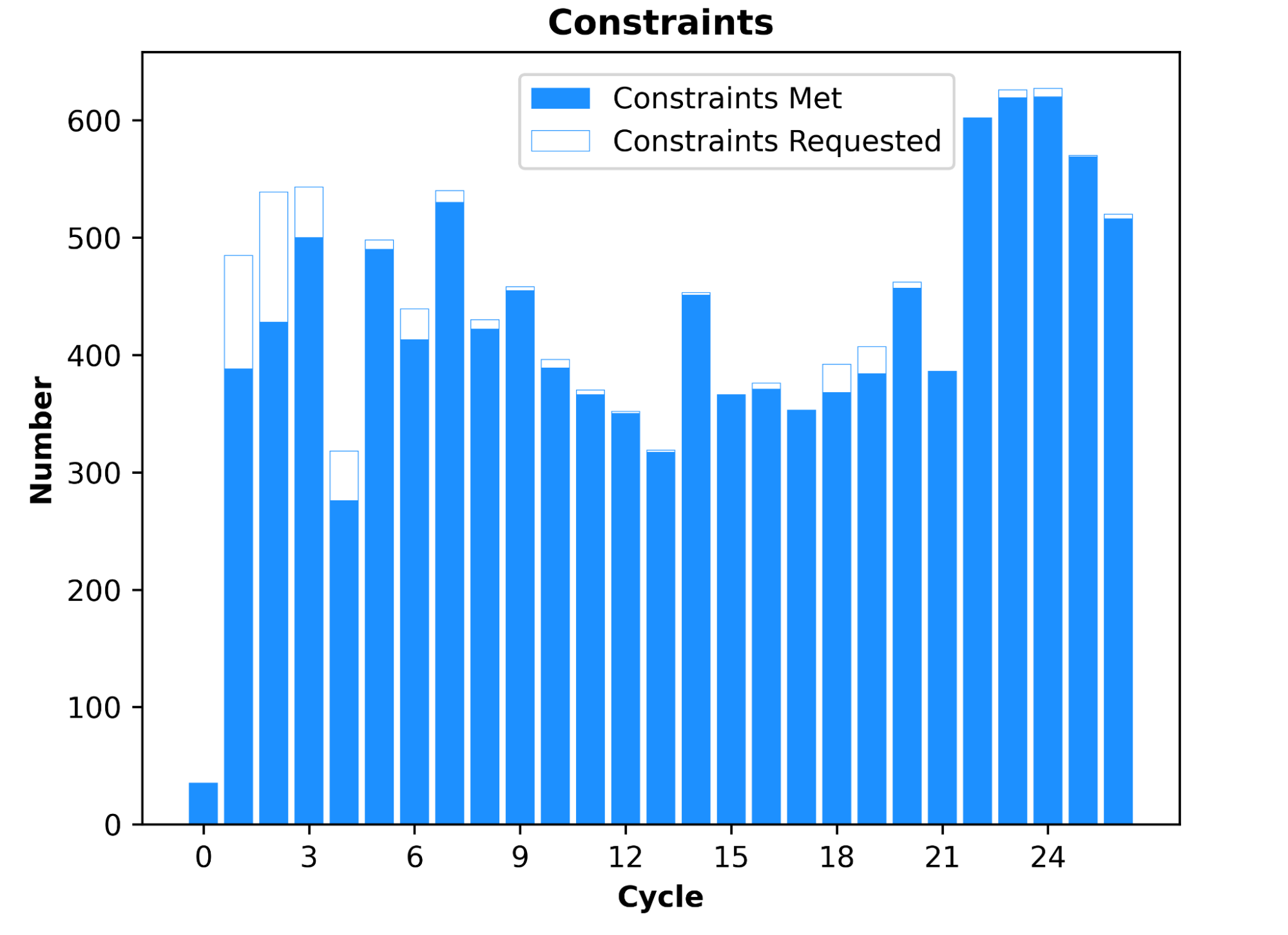
Figure 5: A comparison of constraints requested and constraints met across the history of the mission. The fraction of constraints met is on par with historical values. Violated constraints are dominated by shutdowns, e.g., due to solar flares, and other unavoidable interruptions.
Figure 5 shows the total requested and total met science constraints per cycle across the history of the mission. The figure shows that, despite accepting more science constraints in recent cycles, we continue to meet them with a very high level of success, on par with historical performance. The few missed constraints are dominated by issues such as shutdowns due to solar flares, which cannot be avoided.
Similarly, the historical performance of ToO observations is shown in Figure 6. The blue line shows that the total approved ToO exposure time per cycle has actually, on average, increased with time. However, when the approved time for each program is scaled by its trigger probability, the total "scaled" approved time is roughly flat with time (orange line). The green line shows the observed total ToO exposure time per cycle, which closely matches the scaled approved exposure time. Thus, Chandra's performance with respect to ToO observations remains on par with historical levels.
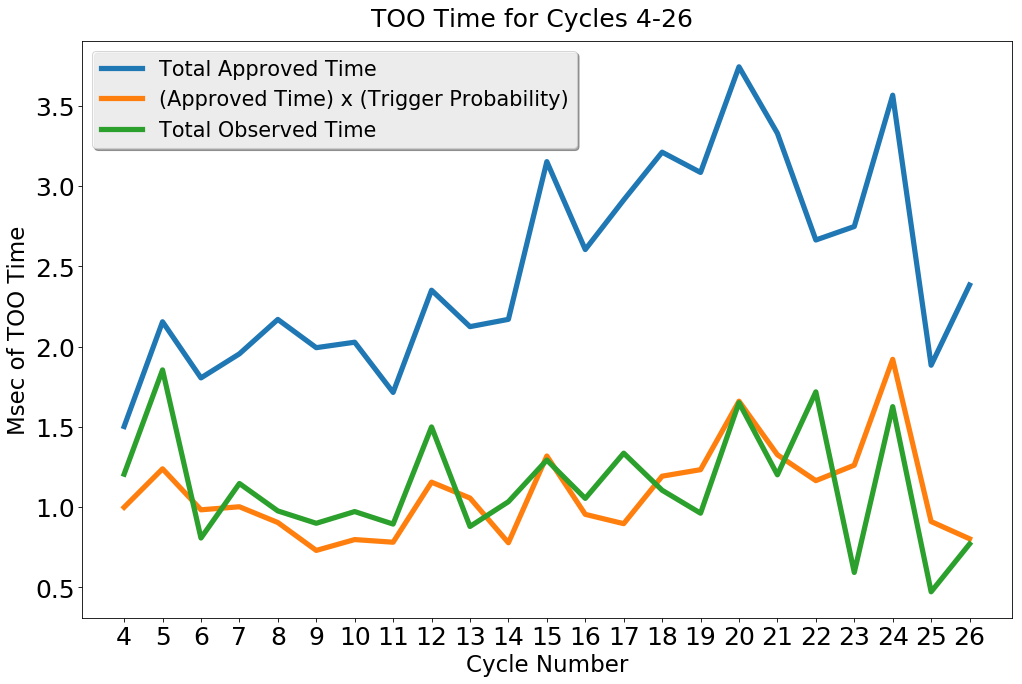
Figure 6: Historical approved and observed ToO time. The blue line shows the total approved time for each cycle. The orange line shows the total approved time times the trigger probability (i.e., the anticipated exposure time), while the green line shows the actual exposure time. The anticipated and actual (orange and green) exposure times are in good agreement and remain, on average, ~1 Msec per cycle over the history of the mission.
Summary
The overall temperature increase of Chandra continues to limit the amount of time we can observe at any given solar pitch angle, due to the temperature limits of the various subsystems. This complicates both constructing the Long Term Schedule and detailed weekly planning and increases the detection threshold of the aspect camera. However, the effects of this heating are mitigated—as much as possible—by several proactive software, procedure, and policy changes, some of which are described in this article. Due to these efforts, and despite increasing challenges, observing metrics remain favorable, with observing efficiency, ToO response, and science constraint compliance that are on par with mission history. There are no known operational barriers to the continued successful and efficient operation of Chandra for years to come.