| PREVIOUS | INDEX | NEXT |
| Focal-Plane Arrays | ||
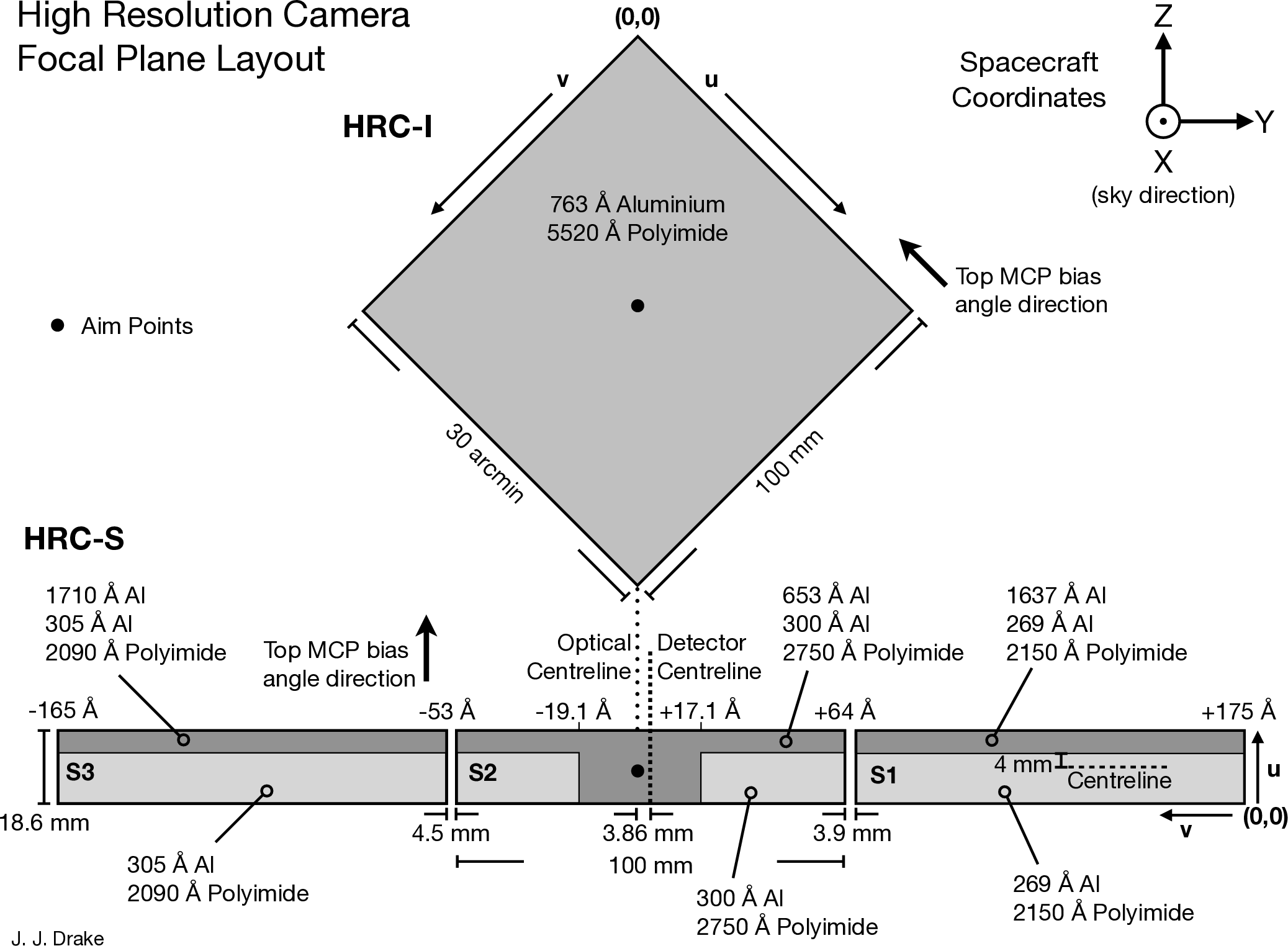
| HRC-I: | CsI-coated MCP pair | 90×90 mm coated |
| (93×93 mm open) | ||
| HRC-S: | CsI-coated MCPpairs | 3-100×20 mm |
| Field of view | HRC-I: | ∼ 30×30 arcmin |
| HRC-S: | 6×99 arcmin | |
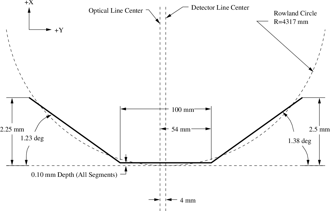
| MCP Bias angle: | 6° | |
| UV/Ion Shields: | ||
| HRC-I: | 5520 Å Polyimide, 763 Å Al | |
| HRC-S: | ||
| Inner segment (S2) | 2750 Å Polyimide, 300 Å Al | |
| Inner segment "T" (S2) | 2750 Å Polyimide, 953 Å Al | |
| Outer segment (S1; +1) | 2150 Å Polyimide, 269 Å Al | |
| Outer segment (LESF) (S1; +1) | 2150 Å Polyimide, 1906 Å Al | |
| Outer segment (S3; −1) | 2090 Å Polyimide, 305 Å Al | |
| Outer segment (LESF) (S3; −1) | 2090 Å Polyimide, 2015 Å Al | |
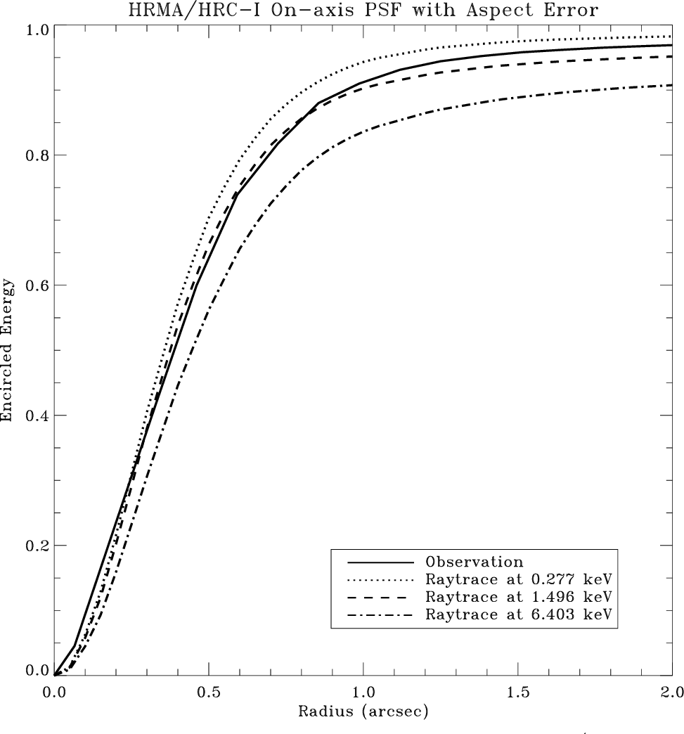
| Spatial resolution | FWHM | ∼ 20μm, ∼ 0.4 arcsec |
| HRC-I: pore size | 10μm | |
| HRC-S: pore size | 12.5μm | |
| HRC-I: pore spacing | 12.5μm | |
| HRC-S: pore spacing | 15μm | |
| pixel size (electronic read-out) | 6.42938μm | |
| [0.13175 arcsec pixel−1] | ||
| pixel size (default binning size) | 0.1318 arcsec pixel−1 | |
| Energy range: | 0.08−10.0 keV | |
| Spectral resolution | ∆E/E | ∼ 1 @1keV |
| MCP Quantum efficiency | 30% @ 1.0 keV | |
| 10% @ 8.0 keV | ||
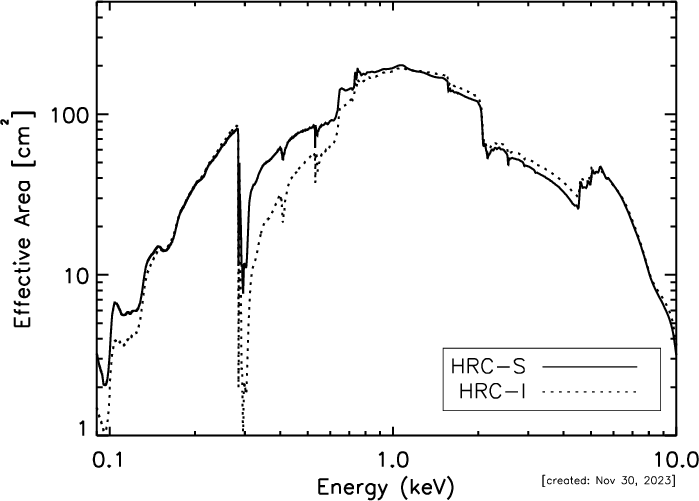
| On-Axis Effective Area: | HRC-I, @ .277 keV | 100 cm2 |
| HRC-I, @ 1 keV | 193 cm2 | |
| HRC-S, @ .277 keV | 85 cm2 | |
| HRC-S, @ 1 keV | 194 cm2 | |
| Time resolution | 16 μsec (see Section 7.12) | |
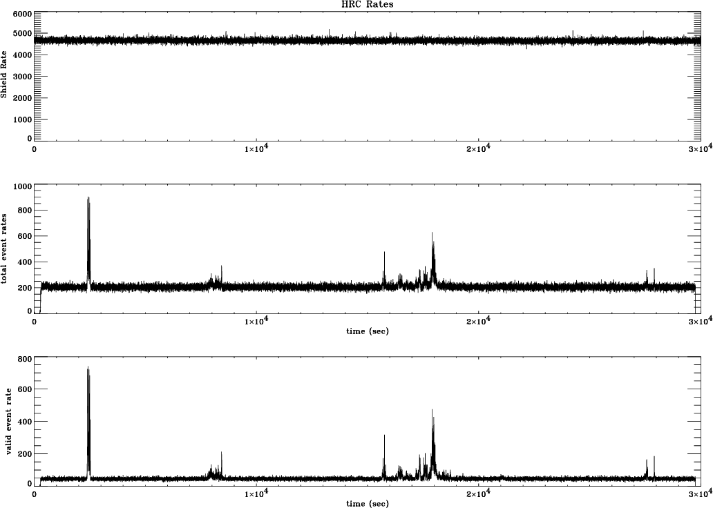
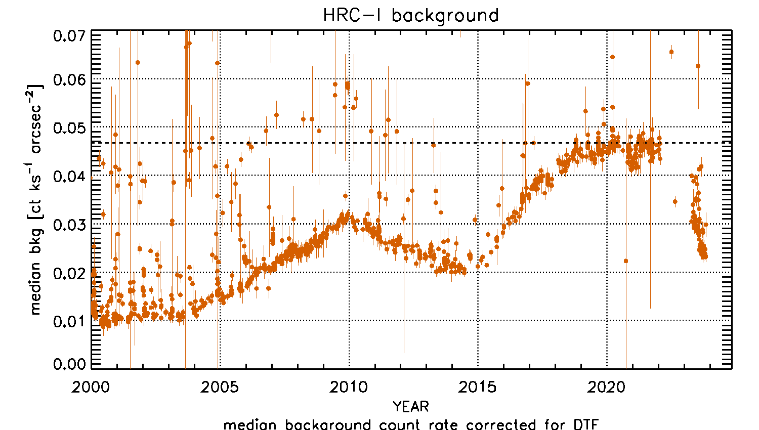
| Expected Quiescent | HRC-I | 3.5×10⁻⁵ cts s−1 arcsec−2 |
| background during Cycle 22 | HRC-S | 7.4×10⁻⁵ cts s−1 arcsec−2 |
| in level 2 data (see Sec 7.11) | ||
| Intrinsic dead time | 50 μs | |
| Constraints: | telemetry limit | 184 cts s−1 |
| maximum counts per aimpoint source | 450000 cts | |
| linearity limit (on-axis point source) | ||
| HRC-I | ∼ 5 cts s−1 (2 cts s−1 pore−1) | |
| HRC-S | ∼ 25 cts s−1 (10 cts s−1 pore−1) |
| (7.1) |
| (7.2) |
| (7.3) |
|
| Model Parameters | NH [×1020 cm−2] | Limiting Fluxf [×10−15 ergs s−1 cm−2] at Background level [counts s−1 arcsec−2] | |||
| 5×10⁻⁶ | 10−5 | 5×10⁻⁵ | 10−4 | ||
| xspowerlaw | |||||
| 0.01 | 6.8 | 8.2 | 17. | 27. | |
| α = 1.4 | 4 | 8.3 | 10. | 21. | 33. |
| 100 | 22. | 27. | 57. | 89. | |
| 0.01 | 5.1 | 6.1 | 13. | 20. | |
| α = 1.7 | 4 | 6.1 | 7.3 | 15. | 24. |
| 100 | 18. | 21. | 45. | 71. | |
| 0.01 | 4.0 | 4.8 | 10. | 16. | |
| α = 2.1 | 4 | 4.4 | 5.2 | 11. | 17. |
| 100 | 13. | 16. | 33. | 52. | |
| 0.01 | 3.8 | 4.6 | 9.7 | 15. | |
| α = 2.4 | 4 | 3.6 | 4.4 | 9.2 | 14. |
| 100 | 11. | 13. | 27. | 42. | |
| xsapec | |||||
| 0.01 | 7.9 | 9.5 | 20. | 32. | |
| kT=0.086 keV | 4 | 3.0 | 3.6 | 7.7 | 12. |
| 100 | 2.0 | 2.4 | 5.0 | 7.8 | |
| 0.01 | 2.0 | 2.4 | 5.0 | 7.8 | |
| kT=0.432 keV | 4 | 1.8 | 2.2 | 4.6 | 7.2 |
| 100 | 2.5 | 3.0 | 6.4 | 10. | |
| 0.01 | 2.3 | 2.8 | 5.8 | 9.2 | |
| kT=0.862 keV | 4 | 2.0 | 2.4 | 5.2 | 8.1 |
| 100 | 3.4 | 4.1 | 8.6 | 13. | |
| 0.01 | 3.4 | 4.1 | 8.6 | 13. | |
| kT=1.72 keV | 4 | 3.3 | 3.9 | 8.2 | 13. |
| 100 | 6.8 | 8.2 | 17. | 27. | |
| Model Parameters | NH [×1020 cm−2] | Limiting Fluxf [×10−15 ergs s−1 cm−2] at Background level [counts s−1 arcsec−2] | |||
| 5×10⁻⁶ | 10−5 | 5×10⁻⁵ | 10−4 | ||
| xspowerlaw | |||||
| 0.01 | 6.7 | 8.1 | 17. | 27. | |
| α = 1.4 | 4 | 8.2 | 9.9 | 21. | 33. |
| 100 | 24. | 29. | 61. | 95. | |
| 0.01 | 4.9 | 5.9 | 12. | 19. | |
| α = 1.7 | 4 | 6.0 | 7.2 | 15. | 24. |
| 100 | 19. | 23. | 48. | 75. | |
| 0.01 | 3.8 | 4.5 | 9.5 | 15. | |
| α = 2.1 | 4 | 4.2 | 5.0 | 11. | 17. |
| 100 | 14. | 17. | 35. | 56. | |
| 0.01 | 3.5 | 4.2 | 8.9 | 14. | |
| α = 2.4 | 4 | 3.4 | 4.1 | 8.6 | 13. |
| 100 | 11. | 14. | 29. | 45. | |
| xsapec | |||||
| 0.01 | 3.5 | 4.2 | 8.9 | 14. | |
| kT=0.086 keV | 4 | 2.5 | 3.0 | 6.3 | 9.9 |
| 100 | 2.0 | 2.3 | 5.0 | 7.8 | |
| 0.01 | 2.0 | 2.4 | 5.2 | 8.1 | |
| kT=0.432 keV | 4 | 1.9 | 2.3 | 4.8 | 7.5 |
| 100 | 2.6 | 3.2 | 6.7 | 10. | |
| 0.01 | 2.3 | 2.8 | 5.9 | 9.2 | |
| kT=0.862 keV | 4 | 2.1 | 2.5 | 5.3 | 8.3 |
| 100 | 3.5 | 4.2 | 8.9 | 14. | |
| 0.01 | 3.3 | 3.9 | 8.2 | 13. | |
| kT=1.72 keV | 4 | 3.2 | 3.8 | 8.1 | 13. |
| 100 | 7.1 | 8.5 | 18. | 28. | |
| Target | Frequency (per Cycle) | Cycle | Grating | Purpose |
| 2REJ1032+532 | 11 | 1 | LETG/None | PSF calibration |
| 31 Com | 1 | > 8 | None | ACIS undercover; off-axis PSF & gain uniformity |
| 3C273 | 1 | 1 | None | Cross-calibration with ACIS |
| AR Lac | 21 | 1-19 | None | Monitor gain at aimpoint & 20 offset locations |
| AR Lac | 42 | 20+ | None | Monitor gain and optical axis at aimpoint & 40 offset locations |
| Betelgeuse | 1 | 3-6 | None | Monitor UV/Ion Shield |
| Capella | 20 | 7-8 | None | Improve de-gap corrections |
| Cen A | 3 | 1 | None | imaging capabilities |
| Cas A | 2 | 1-8 | None | Monitor QE; cross-calibration |
| Cas A | 1/2 | 8-11 | None | Monitor QE; cross-calibration |
| Cas A | 1 | 22 | None | Monitor degap |
| Coma Cluster | 4 | 1 | None | Monitor temporal variations & calibrate de-gap |
| Coma Cluster | 1 | 2,3,16 | None | Monitor temporal variations & calibrate de-gap |
| E0102-72.3 | 1 | 1,14 | None | Cross-calibration with ACIS |
| G21.5-0.9 | 1 | 5-8,19+ | None | Monitor QE; cross-calibration |
| G21.5-0.9 | 2 | 2-4 | None | Monitor QE; cross-calibration |
| G21.5-0.9 | 3 | 0-1 | None | Monitor QE; cross-calibration |
| G21.5-0.9 | 0.5 | 9-18 | None | Monitor QE; cross-calibration |
| HR 1099 | 7 | 20 | None | Monitor PSF size |
| HR 1099 | 1 | 21 | None | Monitor PSF size |
| HR 1099 | 1 | 21 | HETG | Monitor PSF size, calibrate 0th order and HETGS+HRC-I configuration |
| HR 1099 | 63 | 1 | LETG/None | PSF and Wavelength calibration |
| HR 1099 | 30 | 20 | None | PSF calibration |
| HZ 43 | 1 | 8-15 | LETG | Monitor low energy response |
| HZ 43 | 2 | 4-7,16+ | LETG | Monitor low energy response |
| HZ 43 | 3 | 1 | LETG | Monitor low energy response |
| HZ 43 | 4 | 2-3 | LETG | Monitor low energy response |
| LMC X-1 | 16 | 1 | None | PSF calibration |
| M82 | 1 | 1 | None | detector imaging |
| N132D | 2 | 1 | None | Cross-calibration with ACIS |
| NGC 2516 | 3 | 1 | None | Boresighting & plate scale |
| NGC 2516 | 1 | 2 | None | Boresighting & plate scale |
| PKS2155-304 | 2 | 2 | LETG | Monitor low energy QE; cross-calibration |
| PKS2155-304 | 1 | 4 | LETG | Monitor low energy QE; cross-calibration |
| Procyon | 1 | 4-5 | None | ACIS undercover; off-axis PSF & gain uniformity |
| Proxima Cen | 2 | 14,17 | None | ACIS undercover; off-axis PSF & gain uniformity |
| PSRB0540-69 | 5 | 1 | None | Verification of fast timing capability |
| Ross 154 | 1 | 8 | None | ACIS undercover; off-axis PSF & gain uniformity |
| RT Cru | 1 | 14 | None | PSF calibration |
| RXJ1856.5-3754 | 2 | 4-7 | None | ACIS undercover; off-axis PSF & gain uniformity |
| Vega | 2 | 1-7 | None | Monitor UV/Ion Shield |
| Vega | 4 | 7-11 | None | Monitor UV/Ion Shield |
| Vega | 1 | > 11 | None | Monitor UV/Ion Shield |
| Vela SNR | 1 | 3 | None | low energy QE uniformity |
| Vela SNR | 2 | 4 | None | low energy QE uniformity |
| Target | Frequency (per Cycle) | Cycle | Grating | Purpose |
| 3C273 | 1 | 1 | LETG | Cross-calibration |
| 3C273 | 1 | 3 | LETG | Cross-calibration |
| AR Lac | 2x21 | 3,5-8 | None | Monitor gain at aimpoint & 20 offset locations |
| AR Lac | 21 | 1-2,4,9-19 | None | Monitor gain & 20 offset locations |
| AR Lac | 1 | 20+ | None | Monitor gain and PSF at aimpoint |
| AR Lac | 7 | 20 | None | Monitor PSF in cross-dispersion direction |
| Betelgeuse | 4 | 1-6 | None | Monitor UV/Ion Shield |
| Betelgeuse | 2 | 7 | None | Monitor UV/Ion Shield |
| Capella | 10 | 1 | LETG | Monitor gratings |
| Capella | 1 | 1-7,10-13,17+ | LETG | Monitor gratings |
| Cas A | 5 | 1 | None | Cross-calibrate HRC MCPs |
| Cas A | 1/2 | > 9 | None | Cross-calibrate HRC MCPs |
| G21.5-0.9 | 1 | 5-8,15,19 | None | Monitor QE; cross-calibration |
| G21.5-0.9 | 2 | 2,4 | None | Monitor QE; cross-calibration |
| G21.5-0.9 | 3 | 0,3 | None | Monitor QE; cross-calibration |
| G21.5-0.9 | 7 | 1 | None | Monitor QE; cross-calibration |
| G21.5-0.9 | 1 | 24 | LETG | Monitor QE; cross-calibration |
| HR 1099 | 1,21 | 1 | LETG | Wavelength calibration |
| HZ 43 | 1 | 8,10-12,14-15 | LETG | Monitor low energy response |
| HZ 43 | 2 | 0-7,20+ | LETG | Monitor low energy response |
| HZ 43 | 3 | 13,19 | LETG | Monitor low energy response |
| HZ 43 | 4 | 18 | LETG | Monitor low energy response |
| HZ 43 | 14 | 14 | None | Monitor gain across the detector |
| HZ 43 | 16 | 20 | None | Monitor gain across detector, locate thin/thick filter transition |
| LMC X-1 | 26 | 1 | None | PSF calibration |
| Mkn 421 | 1 | 8 | LETG | Monitor ACIS contamination, cross-calibration |
| NGC 2516 | 1 | 1 | None | Boresight and plate-scale |
| PKS2155-304 | 1 | 1-4 | LETG | Gratings calibration, monitor ACIS contamination |
| PKS2155-304 | 2 | 4-8 | LETG | Gratings calibration, monitor ACIS contamination |
| Procyon | 3 | 1 | LETG | Gratings calibration, cross-calibration |
| PSRB0540-69 | 7 | 1 | None | Verification of fast timing capability |
| PSRB1821-24 | 1 | 7 | None | Timing calibration |
| Sirius B | 3 | 1 | LETG | Calibrate LETG low-energy QE |
| Vega | 2x4 | 1-6 | None | Monitor UV/Ion Shield |
| Vega | 4x4 | 6-11 | None | Monitor UV/Ion Shield |
| Vega | 1x4 | > 11 | None | Monitor UV/Ion Shield |
| var. blank sky | ≈ 8 | 22+ | None | Background monitoring at aimpoint during cold ECS pointings |
| PREVIOUS | INDEX | NEXT |