Download the notebook.
Radial profiles, combining, reprojections, and smoothing
Topics
refresher on concepts and terms from yesterday (you all remember what chips ACIS has, don't you?)
a reminder to review the helpful What I Wish I Knew when Starting X-ray Astronomy primer
a (brief) overview on finding and preparing (public) Chandra observations for further analysis
- I do not talk about background flares, which I really should (but Nick has already talked about this)
using
dmextractto create a radial profile (it can also slice - extract spectra - and dice - create light curves)use Sherpa to fit the profile (Aneta will talk more about Sherpa in 45 minutes)
- what features are real, what are instrumental, and what is bad modelling?
if we have more data, we want to combine it to improve our signal-to-noise, but what does that really mean, and why should I care about reprojections, chip boundaries, and instrumental differences?
Unfortunately this is waaaaay to much for a Friday morning, so the idea is to introduce the ideas and point you to the documentation and threads for more details.
The talk
Can we go from
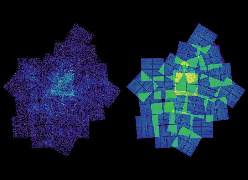
to
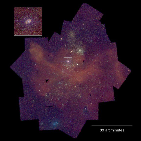
Unfortunately most datasets are just not as pretty as Eta Carina!
Pop Quiz
Can anyone spot the readout streak?
Do we only ever want to combine observations like the Eta Carina dataset? What about the CDF-S datasets?
As the observatory has aged, why do the observation times seem to get smaller?
Let's start by checking the CIAO version (the output of ciaover depends on whether CIAO was installed with
ciao-install or conda; in this case I used conda):
!ciaover -v
# packages in environment at /home/dburke/anaconda/envs/ciao413:
#
# Name                    Version                   Build  Channel
ciao                      4.13.0           py38h5ec60c1_0    https://cxc.cfa.harvard.edu/conda/ciao
ciao-contrib              4.13.0                     py_4    https://cxc.cfa.harvard.edu/conda/ciao
ds9                       8.2                           2    https://cxc.cfa.harvard.edu/conda/ciao
sherpa                    4.13.0           py38h5ec60c1_0    https://cxc.cfa.harvard.edu/conda/ciao

System information:
Linux dburke-Precision-5530 5.4.0-59-generic #65-Ubuntu SMP Thu Dec 10 12:01:51 UTC 2020 x86_64 x86_64 x86_64 GNU/Linux
For this talk I am using an IPython notebook, but running many commands via the shell (by starting a line with the ! character). To save time I will not run all steps in the talk.
I want data on the $z \sim 1$ galaxy cluster around the QSO 3C 186. Let's search the Chandra archive:
!find_chandra_obsid '3C 186'
# obsid  sepn   inst grat   time    obsdate        piname    target
3098      0.0 ACIS-S NONE   34.4 2002-05-16 Siemiginowska Q0740+380
9407      0.0 ACIS-S NONE   66.3 2007-12-03 Siemiginowska  "3C 186"
9408      0.0 ACIS-S NONE   39.6 2007-12-11 Siemiginowska  "3C 186"
9774      0.0 ACIS-S NONE   75.1 2007-12-06 Siemiginowska  "3C 186"
9775      0.0 ACIS-S NONE   15.9 2007-12-08 Siemiginowska  "3C 186"
The fact that the PI is the same person who is giving you the next talk is purely coincidental, as is our 2010 paper on this cluster you can read ...
Pop Quiz time
What's an ObsId?
What does ACIS-S mean?
Why is the observation date important?
Is the target field meaningfull?
So, there was a "short" observation in 2002 and then ~200 ks of data in 2007. Let's grab them all (it can take a bit of time, so
download_chandra_obsid 9774can be used to access just a single ObsId). Apologies for the wall of text here!
!mkdir data
cd data
/home/dburke/talks/ciao_workshop_jan_21_aas237/notebooks/data
!find_chandra_obsid '3C 186' download=all
Downloading files for ObsId 3098, total size is 99 Mb.

  Type     Format      Size  0........H.........1  Download Time Average Rate
  ---------------------------------------------------------------------------
  vv       pdf        73 Mb  ####################           43 s  1739.2 kb/s
  asol     fits        9 Mb  ####################            7 s  1453.1 kb/s
  mtl      fits        8 Mb  ####################            2 s  4194.7 kb/s
  evt1     fits        3 Mb  ####################          < 1 s  4289.2 kb/s
  stat     fits        1 Mb  ####################          < 1 s  1612.0 kb/s
  evt2     fits        1 Mb  ####################          < 1 s  2127.4 kb/s
  aqual    fits      570 Kb  ####################          < 1 s  1388.5 kb/s
  osol     fits      366 Kb  ####################          < 1 s  1219.3 kb/s
  osol     fits      361 Kb  ####################          < 1 s  1141.3 kb/s
  osol     fits      352 Kb  ####################          < 1 s  1054.3 kb/s
  osol     fits      351 Kb  ####################          < 1 s  776.4 kb/s
  osol     fits      350 Kb  ####################          < 1 s  1339.7 kb/s
  osol     fits      350 Kb  ####################          < 1 s  934.0 kb/s
  eph1     fits      282 Kb  ####################          < 1 s  549.6 kb/s
  eph1     fits      275 Kb  ####################          < 1 s  832.1 kb/s
  eph1     fits      253 Kb  ####################          < 1 s  637.2 kb/s
  osol     fits      167 Kb  ####################          < 1 s  619.8 kb/s
  cntr_img jpg       110 Kb  ####################          < 1 s  187.4 kb/s
  bias     fits       71 Kb  ####################          < 1 s  261.7 kb/s
  cntr_img fits       40 Kb  ####################          < 1 s  198.9 kb/s
  vv       pdf        30 Kb  ####################          < 1 s  209.9 kb/s
  oif      fits       23 Kb  ####################          < 1 s  130.3 kb/s
  eph1     fits       15 Kb  ####################          < 1 s  54.2 kb/s
  full_img fits       13 Kb  ####################          < 1 s  43.3 kb/s
  readme   ascii      10 Kb  ####################          < 1 s  51.4 kb/s
  fov      fits        5 Kb  ####################          < 1 s  24.0 kb/s
  flt      fits        5 Kb  ####################          < 1 s  22.1 kb/s
  bpix     fits        4 Kb  ####################          < 1 s  21.1 kb/s
  msk      fits        4 Kb  ####################          < 1 s  23.2 kb/s
  pbk      fits        4 Kb  ####################          < 1 s  25.3 kb/s
  full_img jpg         2 Kb  ####################          < 1 s  8.6 kb/s

      Total download size for ObsId 3098 = 99 Mb
      Total download time for ObsId 3098 = 1 m 1 s

Downloading files for ObsId 9407, total size is 379 Mb.

  Type     Format      Size  0........H.........1  Download Time Average Rate
  ---------------------------------------------------------------------------
  evt1     fits      193 Mb  ####################       1 m 36 s  2060.2 kb/s
  vv       pdf       128 Mb  ####################        1 m 7 s  1957.4 kb/s
  evt2     fits       28 Mb  ####################           14 s  2025.7 kb/s
  asol     fits       16 Mb  ####################            8 s  2165.7 kb/s
  mtl      fits        3 Mb  ####################            1 s  2132.1 kb/s
  stat     fits        2 Mb  ####################          < 1 s  3667.1 kb/s
  aqual    fits     1011 Kb  ####################          < 1 s  2152.8 kb/s
  bias     fits      496 Kb  ####################          < 1 s  701.6 kb/s
  cntr_img jpg       474 Kb  ####################          < 1 s  755.3 kb/s
  bias     fits      453 Kb  ####################          < 1 s  646.0 kb/s
  bias     fits      442 Kb  ####################          < 1 s  852.4 kb/s
  bias     fits      442 Kb  ####################          < 1 s  1405.1 kb/s
  bias     fits      440 Kb  ####################          < 1 s  633.4 kb/s
  osol     fits      366 Kb  ####################          < 1 s  1096.8 kb/s
  osol     fits      359 Kb  ####################          < 1 s  1452.1 kb/s
  osol     fits      353 Kb  ####################          < 1 s  1461.7 kb/s
  osol     fits      349 Kb  ####################          < 1 s  568.2 kb/s
  osol     fits      349 Kb  ####################          < 1 s  655.9 kb/s
  osol     fits      348 Kb  ####################          < 1 s  877.7 kb/s
  osol     fits      348 Kb  ####################          < 1 s  581.6 kb/s
  osol     fits      348 Kb  ####################          < 1 s  880.8 kb/s
  osol     fits      348 Kb  ####################          < 1 s  1004.7 kb/s
  osol     fits      348 Kb  ####################          < 1 s  566.5 kb/s
  osol     fits      347 Kb  ####################          < 1 s  737.2 kb/s
  eph1     fits      283 Kb  ####################          < 1 s  455.0 kb/s
  eph1     fits      276 Kb  ####################          < 1 s  1240.8 kb/s
  eph1     fits      258 Kb  ####################          < 1 s  1336.7 kb/s
  cntr_img fits      226 Kb  ####################          < 1 s  1006.7 kb/s
  osol     fits      198 Kb  ####################          < 1 s  740.3 kb/s
  osol     fits      110 Kb  ####################          < 1 s  509.2 kb/s
  full_img fits       80 Kb  ####################          < 1 s  382.1 kb/s
  bpix     fits       58 Kb  ####################          < 1 s  249.1 kb/s
  full_img jpg        44 Kb  ####################          < 1 s  156.1 kb/s
  vv       pdf        38 Kb  ####################          < 1 s  172.4 kb/s
  oif      fits       25 Kb  ####################          < 1 s  100.2 kb/s
  eph1     fits       24 Kb  ####################          < 1 s  221.8 kb/s
  readme   ascii      10 Kb  ####################          < 1 s  113.7 kb/s
  flt      fits        7 Kb  ####################          < 1 s  71.8 kb/s
  fov      fits        6 Kb  ####################          < 1 s  63.5 kb/s
  msk      fits        5 Kb  ####################          < 1 s  32.0 kb/s
  pbk      fits        4 Kb  ####################          < 1 s  12.5 kb/s

      Total download size for ObsId 9407 = 379 Mb
      Total download time for ObsId 9407 = 3 m 19 s

Downloading files for ObsId 9408, total size is 228 Mb.

  Type     Format      Size  0........H.........1  Download Time Average Rate
  ---------------------------------------------------------------------------
  evt1     fits      114 Mb  ####################       1 m 13 s  1587.8 kb/s
  vv       pdf        78 Mb  ####################           54 s  1490.8 kb/s
  evt2     fits       17 Mb  ####################            4 s  4038.9 kb/s
  asol     fits       10 Mb  ####################            2 s  5326.0 kb/s
  mtl      fits        2 Mb  ####################          < 1 s  2741.5 kb/s
  stat     fits        1 Mb  ####################          < 1 s  2382.7 kb/s
  aqual    fits      609 Kb  ####################          < 1 s  1564.8 kb/s
  cntr_img jpg       519 Kb  ####################          < 1 s  1544.8 kb/s
  bias     fits      499 Kb  ####################          < 1 s  945.0 kb/s
  bias     fits      454 Kb  ####################          < 1 s  944.5 kb/s
  bias     fits      443 Kb  ####################          < 1 s  1032.3 kb/s
  bias     fits      439 Kb  ####################          < 1 s  1123.5 kb/s
  bias     fits      438 Kb  ####################          < 1 s  537.9 kb/s
  osol     fits      358 Kb  ####################          < 1 s  860.1 kb/s
  osol     fits      356 Kb  ####################          < 1 s  880.7 kb/s
  osol     fits      351 Kb  ####################          < 1 s  663.8 kb/s
  osol     fits      350 Kb  ####################          < 1 s  1123.5 kb/s
  osol     fits      348 Kb  ####################          < 1 s  387.4 kb/s
  osol     fits      348 Kb  ####################          < 1 s  817.8 kb/s
  osol     fits      347 Kb  ####################          < 1 s  776.8 kb/s
  eph1     fits      283 Kb  ####################          < 1 s  506.6 kb/s
  eph1     fits      277 Kb  ####################          < 1 s  665.4 kb/s
  eph1     fits      259 Kb  ####################          < 1 s  1084.6 kb/s
  cntr_img fits      168 Kb  ####################          < 1 s  594.9 kb/s
  osol     fits       98 Kb  ####################          < 1 s  365.1 kb/s
  osol     fits       90 Kb  ####################          < 1 s  522.0 kb/s
  full_img fits       73 Kb  ####################          < 1 s  299.1 kb/s
  full_img jpg        47 Kb  ####################          < 1 s  275.9 kb/s
  bpix     fits       43 Kb  ####################          < 1 s  233.0 kb/s
  vv       pdf        37 Kb  ####################          < 1 s  237.8 kb/s
  oif      fits       25 Kb  ####################          < 1 s  187.8 kb/s
  eph1     fits       16 Kb  ####################          < 1 s  118.7 kb/s
  readme   ascii      10 Kb  ####################          < 1 s  71.5 kb/s
  flt      fits        7 Kb  ####################          < 1 s  32.4 kb/s
  fov      fits        6 Kb  ####################          < 1 s  28.6 kb/s
  msk      fits        5 Kb  ####################          < 1 s  36.6 kb/s
  pbk      fits        4 Kb  ####################          < 1 s  21.5 kb/s

      Total download size for ObsId 9408 = 228 Mb
      Total download time for ObsId 9408 = 2 m 25 s

Downloading files for ObsId 9774, total size is 432 Mb.

  Type     Format      Size  0........H.........1  Download Time Average Rate
  ---------------------------------------------------------------------------
  evt1     fits      222 Mb  ####################        2 m 9 s  1758.7 kb/s
  vv       pdf       145 Mb  ####################       1 m 15 s  1974.6 kb/s
  evt2     fits       32 Mb  ####################           16 s  2077.1 kb/s
  asol     fits       19 Mb  ####################            5 s  3982.9 kb/s
  mtl      fits        3 Mb  ####################          < 1 s  5733.5 kb/s
  stat     fits        2 Mb  ####################          < 1 s  3769.3 kb/s
  aqual    fits        1 Mb  ####################          < 1 s  4168.1 kb/s
  bias     fits      495 Kb  ####################          < 1 s  1937.3 kb/s
  cntr_img jpg       487 Kb  ####################          < 1 s  1508.5 kb/s
  bias     fits      453 Kb  ####################          < 1 s  1427.5 kb/s
  bias     fits      448 Kb  ####################          < 1 s  1630.6 kb/s
  bias     fits      442 Kb  ####################          < 1 s  1342.7 kb/s
  bias     fits      439 Kb  ####################          < 1 s  1536.5 kb/s
  osol     fits      359 Kb  ####################          < 1 s  1416.4 kb/s
  osol     fits      354 Kb  ####################          < 1 s  1413.6 kb/s
  osol     fits      349 Kb  ####################          < 1 s  1373.8 kb/s
  osol     fits      349 Kb  ####################          < 1 s  1251.6 kb/s
  osol     fits      349 Kb  ####################          < 1 s  1435.7 kb/s
  osol     fits      349 Kb  ####################          < 1 s  1413.9 kb/s
  osol     fits      349 Kb  ####################          < 1 s  1456.4 kb/s
  osol     fits      348 Kb  ####################          < 1 s  1191.6 kb/s
  osol     fits      348 Kb  ####################          < 1 s  1181.7 kb/s
  osol     fits      348 Kb  ####################          < 1 s  1379.2 kb/s
  osol     fits      348 Kb  ####################          < 1 s  1302.2 kb/s
  eph1     fits      283 Kb  ####################          < 1 s  908.9 kb/s
  eph1     fits      276 Kb  ####################          < 1 s  975.8 kb/s
  osol     fits      273 Kb  ####################          < 1 s  638.5 kb/s
  osol     fits      268 Kb  ####################          < 1 s  788.6 kb/s
  eph1     fits      258 Kb  ####################          < 1 s  607.6 kb/s
  cntr_img fits      242 Kb  ####################          < 1 s  692.9 kb/s
  osol     fits      148 Kb  ####################          < 1 s  439.1 kb/s
  osol     fits       97 Kb  ####################          < 1 s  348.3 kb/s
  full_img fits       82 Kb  ####################          < 1 s  411.0 kb/s
  bpix     fits       62 Kb  ####################          < 1 s  302.7 kb/s
  full_img jpg        45 Kb  ####################          < 1 s  376.3 kb/s
  vv       pdf        38 Kb  ####################          < 1 s  343.5 kb/s
  eph1     fits       26 Kb  ####################          < 1 s  208.0 kb/s
  oif      fits       25 Kb  ####################          < 1 s  164.5 kb/s
  osol     fits       19 Kb  ####################          < 1 s  151.4 kb/s
  readme   ascii      10 Kb  ####################          < 1 s  95.4 kb/s
  flt      fits        7 Kb  ####################          < 1 s  62.4 kb/s
  fov      fits        6 Kb  ####################          < 1 s  28.5 kb/s
  msk      fits        5 Kb  ####################          < 1 s  18.4 kb/s
  pbk      fits        4 Kb  ####################          < 1 s  20.6 kb/s

      Total download size for ObsId 9774 = 432 Mb
      Total download time for ObsId 9774 = 3 m 55 s

Downloading files for ObsId 9775, total size is 99 Mb.

  Type     Format      Size  0........H.........1  Download Time Average Rate
  ---------------------------------------------------------------------------
  evt1     fits       48 Mb  ####################           26 s  1853.2 kb/s
  vv       pdf        33 Mb  ####################           21 s  1591.1 kb/s
  evt2     fits        7 Mb  ####################          < 1 s  10556.8 kb/s
  asol     fits        4 Mb  ####################            1 s  2977.3 kb/s
  mtl      fits      694 Kb  ####################          < 1 s  3772.3 kb/s
  cntr_img jpg       536 Kb  ####################          < 1 s  2075.3 kb/s
  stat     fits      499 Kb  ####################          < 1 s  2634.4 kb/s
  bias     fits      495 Kb  ####################          < 1 s  2576.8 kb/s
  bias     fits      450 Kb  ####################          < 1 s  2136.4 kb/s
  bias     fits      448 Kb  ####################          < 1 s  2113.4 kb/s
  bias     fits      447 Kb  ####################          < 1 s  2239.3 kb/s
  bias     fits      444 Kb  ####################          < 1 s  2428.4 kb/s
  osol     fits      365 Kb  ####################          < 1 s  2060.5 kb/s
  osol     fits      361 Kb  ####################          < 1 s  1875.7 kb/s
  osol     fits      353 Kb  ####################          < 1 s  1876.3 kb/s
  osol     fits      348 Kb  ####################          < 1 s  1952.9 kb/s
  eph1     fits      283 Kb  ####################          < 1 s  1551.1 kb/s
  eph1     fits      277 Kb  ####################          < 1 s  1579.8 kb/s
  eph1     fits      259 Kb  ####################          < 1 s  1462.5 kb/s
  aqual    fits      251 Kb  ####################          < 1 s  1443.5 kb/s
  cntr_img fits      102 Kb  ####################          < 1 s  653.6 kb/s
  full_img fits       61 Kb  ####################          < 1 s  447.8 kb/s
  full_img jpg        54 Kb  ####################          < 1 s  428.3 kb/s
  vv       pdf        35 Kb  ####################          < 1 s  327.2 kb/s
  bpix     fits       26 Kb  ####################          < 1 s  221.5 kb/s
  oif      fits       23 Kb  ####################          < 1 s  148.3 kb/s
  readme   ascii      10 Kb  ####################          < 1 s  82.1 kb/s
  eph1     fits        8 Kb  ####################          < 1 s  68.8 kb/s
  flt      fits        7 Kb  ####################          < 1 s  43.8 kb/s
  fov      fits        6 Kb  ####################          < 1 s  42.1 kb/s
  msk      fits        5 Kb  ####################          < 1 s  40.5 kb/s
  pbk      fits        4 Kb  ####################          < 1 s  26.2 kb/s

      Total download size for ObsId 9775 = 99 Mb
      Total download time for ObsId 9775 = 55 s
Pop Quiz
What are all these different "types"?
What ones should I care about?
What's the first file I should review?
This has created five directories, one for each ObsId:
!ls
3098 9407 9408 9774 9775
!punlearn chandra_repro
!plist chandra_repro
Parameters for /home/dburke/cxcds_param4/chandra_repro.par

         indir = ./               Input directory
        outdir =                  Output directory (default = $indir/repro)
         (root = )                Root for output filenames
     (badpixel = yes)             Create a new bad pixel file?
(process_events = yes)             Create a new level=2 event file?
     (destreak = yes)             Destreak the ACIS-8 chip?
   (set_ardlib = yes)             Set ardlib.par with the bad pixel file?
 (check_vf_pha = no)              Clean ACIS background in VFAINT data?
      (pix_adj = default)         Pixel randomization: default|edser|none|randomize
(recreate_tg_mask = no)              Re-run tgdetect and tg_create_mask rather than use the Level 2 region extension?
  (asol_update = yes)             If necessary, apply boresight correction to aspect solution file?
      (cleanup = yes)             Cleanup intermediate files on exit
      (clobber = no)              Clobber existing file
      (verbose = 1)               Debug Level(0-5)
         (mode = ql)
!chandra_repro indir=* outdir=
Running chandra_repro
version: 01 December 2020

WARNING: "set_ardlib=yes" cannot be used with multiple input directories.  Changing to "no"


Processing input directory '/home/dburke/talks/ciao_workshop_jan_21_aas237/notebooks/data/3098'

Applying boresight update to aspect solution file
Resetting afterglow status bits in evt1.fits file...

Running acis_build_badpix and acis_find_afterglow to create a new bad pixel file...

Running acis_process_events to reprocess the evt1.fits file...
Output from acis_process_events:
# acis_process_events (CIAO 4.13): WARNING: The ra_targ, dec_targ, or roll_nom specified by /home/dburke/talks/ciao_workshop_jan_21_aas237/notebooks/data/3098/repro/pcadf03098_repro_obs.par does not match the values in the event file- using the obs.par values.
Filtering the evt1.fits file by grade and status and time...
Applying the good time intervals from the flt1.fits file...
The new evt2.fits file is: /home/dburke/talks/ciao_workshop_jan_21_aas237/notebooks/data/3098/repro/acisf03098_repro_evt2.fits

Updating the event file header with chandra_repro HISTORY record
Creating FOV file...

Cleaning up intermediate files

The data have been reprocessed.
Start your analysis with the new products in
/home/dburke/talks/ciao_workshop_jan_21_aas237/notebooks/data/3098/repro


Processing input directory '/home/dburke/talks/ciao_workshop_jan_21_aas237/notebooks/data/9407'

Applying boresight update to aspect solution file
Resetting afterglow status bits in evt1.fits file...

Running acis_build_badpix and acis_find_afterglow to create a new bad pixel file...

Running acis_process_events to reprocess the evt1.fits file...
Output from acis_process_events:
# acis_process_events (CIAO 4.13): WARNING: The ra_targ, dec_targ, or roll_nom specified by /home/dburke/talks/ciao_workshop_jan_21_aas237/notebooks/data/9407/repro/pcadf09407_repro_obs.par does not match the values in the event file- using the obs.par values.
# acis_process_events (CIAO 4.13): The following error occurred 13 times:
	dsAPEPULSEHEIGHTERR -- WARNING: pulse height is less than split threshold when performing serial CTI adjustment.
Filtering the evt1.fits file by grade and status and time...
Applying the good time intervals from the flt1.fits file...
The new evt2.fits file is: /home/dburke/talks/ciao_workshop_jan_21_aas237/notebooks/data/9407/repro/acisf09407_repro_evt2.fits

Updating the event file header with chandra_repro HISTORY record
Creating FOV file...

Cleaning up intermediate files

The data have been reprocessed.
Start your analysis with the new products in
/home/dburke/talks/ciao_workshop_jan_21_aas237/notebooks/data/9407/repro


Processing input directory '/home/dburke/talks/ciao_workshop_jan_21_aas237/notebooks/data/9408'

Applying boresight update to aspect solution file
Resetting afterglow status bits in evt1.fits file...

Running acis_build_badpix and acis_find_afterglow to create a new bad pixel file...

Running acis_process_events to reprocess the evt1.fits file...
Output from acis_process_events:
# acis_process_events (CIAO 4.13): WARNING: The ra_targ, dec_targ, or roll_nom specified by /home/dburke/talks/ciao_workshop_jan_21_aas237/notebooks/data/9408/repro/pcadf09408_repro_obs.par does not match the values in the event file- using the obs.par values.
# acis_process_events (CIAO 4.13): The following error occurred 4 times:
	dsAPEPULSEHEIGHTERR -- WARNING: pulse height is less than split threshold when performing serial CTI adjustment.
Filtering the evt1.fits file by grade and status and time...
Applying the good time intervals from the flt1.fits file...
The new evt2.fits file is: /home/dburke/talks/ciao_workshop_jan_21_aas237/notebooks/data/9408/repro/acisf09408_repro_evt2.fits

Updating the event file header with chandra_repro HISTORY record
Creating FOV file...

Cleaning up intermediate files

The data have been reprocessed.
Start your analysis with the new products in
/home/dburke/talks/ciao_workshop_jan_21_aas237/notebooks/data/9408/repro


Processing input directory '/home/dburke/talks/ciao_workshop_jan_21_aas237/notebooks/data/9774'

Applying boresight update to aspect solution file
Resetting afterglow status bits in evt1.fits file...

Running acis_build_badpix and acis_find_afterglow to create a new bad pixel file...

Running acis_process_events to reprocess the evt1.fits file...
Output from acis_process_events:
# acis_process_events (CIAO 4.13): WARNING: The ra_targ, dec_targ, or roll_nom specified by /home/dburke/talks/ciao_workshop_jan_21_aas237/notebooks/data/9774/repro/pcadf09774_repro_obs.par does not match the values in the event file- using the obs.par values.
# acis_process_events (CIAO 4.13): The following error occurred 13 times:
	dsAPEPULSEHEIGHTERR -- WARNING: pulse height is less than split threshold when performing serial CTI adjustment.
Filtering the evt1.fits file by grade and status and time...
Applying the good time intervals from the flt1.fits file...
The new evt2.fits file is: /home/dburke/talks/ciao_workshop_jan_21_aas237/notebooks/data/9774/repro/acisf09774_repro_evt2.fits

Updating the event file header with chandra_repro HISTORY record
Creating FOV file...

Cleaning up intermediate files

The data have been reprocessed.
Start your analysis with the new products in
/home/dburke/talks/ciao_workshop_jan_21_aas237/notebooks/data/9774/repro


Processing input directory '/home/dburke/talks/ciao_workshop_jan_21_aas237/notebooks/data/9775'

Applying boresight update to aspect solution file
Resetting afterglow status bits in evt1.fits file...

Running acis_build_badpix and acis_find_afterglow to create a new bad pixel file...

Running acis_process_events to reprocess the evt1.fits file...
Output from acis_process_events:
# acis_process_events (CIAO 4.13): WARNING: The ra_targ, dec_targ, or roll_nom specified by /home/dburke/talks/ciao_workshop_jan_21_aas237/notebooks/data/9775/repro/pcadf09775_repro_obs.par does not match the values in the event file- using the obs.par values.
# acis_process_events (CIAO 4.13): The following error occurred 3 times:
	dsAPEPULSEHEIGHTERR -- WARNING: pulse height is less than split threshold when performing serial CTI adjustment.
Filtering the evt1.fits file by grade and status and time...
Applying the good time intervals from the flt1.fits file...
The new evt2.fits file is: /home/dburke/talks/ciao_workshop_jan_21_aas237/notebooks/data/9775/repro/acisf09775_repro_evt2.fits

Updating the event file header with chandra_repro HISTORY record
Creating FOV file...

Cleaning up intermediate files

The data have been reprocessed.
Start your analysis with the new products in
/home/dburke/talks/ciao_workshop_jan_21_aas237/notebooks/data/9775/repro
NOTE New to CIAO 4.13 is the helpful WARNING message
The ra_targ, dec_targ, or roll_nom specified by /blah/blah/blah_obs.par does not match the values in the event file- using the obs.par values.This is thanks to a new correction to handle changes in our understanding of the alignment of the telescope and can (at least here), be ignored.
Pop Quiz
Rember virtual filtering?
!dmstat 9774/repro/acisf09774_repro_evt2.fits"[ccd_id=3,sky=circle(4100,4100,30)][cols energy]"
# DMSTAT (CIAO 4.13): WARNING: no rows found in table 9774/repro/acisf09774_repro_evt2.fits[ccd_id=3,sky=circle(4100,4100,30)][cols energy]

energy[eV]
    min:	0 	      @:	0
    max:	0 	      @:	0
   mean:	0
  sigma:	0
    sum:	0
   good:	0
   null:	0
Darn it - I meant ccd_id=7...
What does the data look like?
We can use the fluximage script to create exposure-map corrected images (as with chandra_repro this packages up a numbre of different tasks that call CIAO commands):
!punlearn fluximage
!fluximage 9774/ 9774/fluxed/
Running fluximage
Version: 01 April 2020

Found 9774/repro/acisf09774_repro_evt2.fits
Using event file 9774/repro/acisf09774_repro_evt2.fits
Using CSC ACIS broad science energy band.
Aspect solution 9774/repro/pcadf09774_repro_asol1.fits found.
Bad-pixel file 9774/repro/acisf09774_repro_bpix1.fits found.
Mask file 9774/repro/acisf09774_000N002_msk1.fits found.

The output images will have 386 by 412 pixels, pixel size of 3.936 arcsec,
    and cover x=2056.5:5144.5:8,y=3176.5:6472.5:8.

Running tasks in parallel with 12 processors.
Creating aspect histograms for obsid 9774
Creating 5 instrument maps for obsid 9774
Creating 5 exposure maps for obsid 9774
Combining 5 exposure maps for obsid 9774
Thresholding data for obsid 9774
Exposure-correcting image for obsid 9774

The following files were created:

 The clipped counts image is:
     9774/fluxed/broad_thresh.img

 The clipped exposure map is:
     9774/fluxed/broad_thresh.expmap

 The exposure-corrected image is:
     9774/fluxed/broad_flux.img
You can use ds9 to view these, but it doesn't work well in a shared notebook, so let's display
it within the notebook using crated (to read the data) and matlotlib (to display the data):
import numpy as np
from matplotlib import pyplot as plt
import pycrates

%matplotlib inline
cr = pycrates.read_file('9774/fluxed/broad_thresh.img')
pixvals = cr.get_image().values
plt.figure(figsize=(8, 8))
plt.imshow(pixvals, origin='lower')
<matplotlib.image.AxesImage at 0x7ff0e0f86fd0>
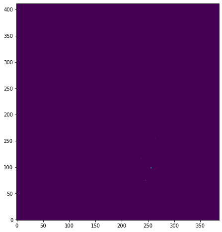
Well, that doesn't lool very pretty. How about using a log scale?
plt.figure(figsize=(8, 8))
plt.imshow(np.log10(pixvals), origin='lower')
<ipython-input-15-67ead6e88e68>:2: RuntimeWarning: divide by zero encountered in log10
  plt.imshow(np.log10(pixvals), origin='lower')
<matplotlib.image.AxesImage at 0x7ff0e07b0a60>
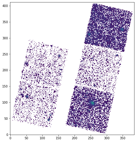
Pop Quiz
Can you identify the chips?
Why are two of the chips so-much brighter than the others?
In fact, what data is being shown here?
what do the bins represent
what are the axes
from coords.resolver import identify_name

pos = identify_name('3C 186')
print(pos)
(20.46333333, 33.2825, 'ICRS')
Since this is a python notebook (not a bash one like in Kenny's example) we can't quite use the same tricks for running ds9 in the background.
Let's look at the "counts" image (this takes too long to run over zoom so images have been added to show the output):
!ds9 9774/fluxed/broad_thresh.img -pan to 116.07272 37.88809722 ICRS \
  -zoom 4 -scale log
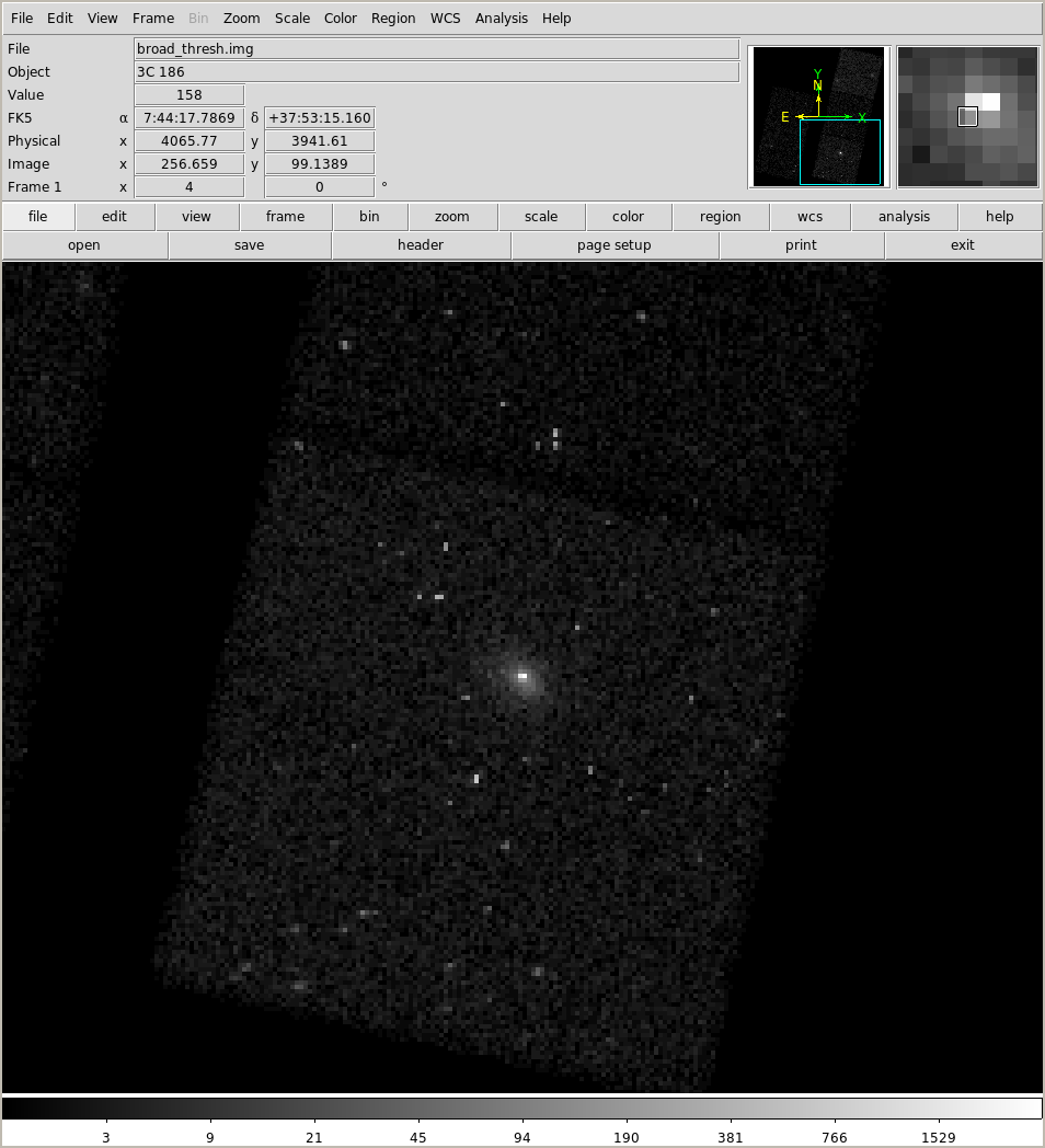
NOTE 1 you must exit ds9 otherwise the newer notebook cells will not run!
NOTE 2 I am displaying an image, not an events file, so you don't get the "missing data" that Kenny mentioned in the start of his DS9 overview.
Now for the "flux" image (which is the counts image divided by the exposure map):
!ds9 9774/fluxed/broad_flux.img -pan to 116.07272 37.88809722 ICRS \
  -zoom 4 -scale log
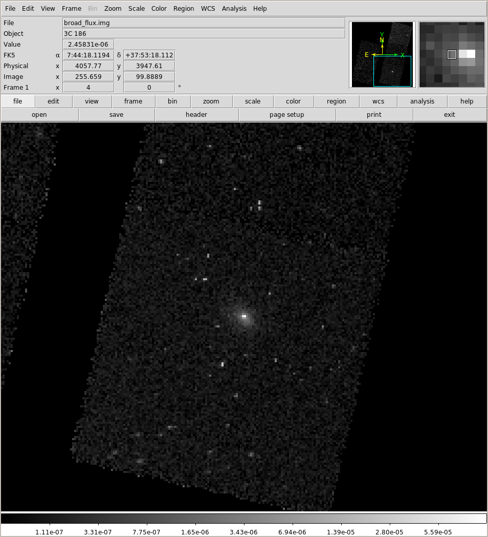
NOTE this is the "fluxed" image which reduces - but does not eliminate - the impact of chip boundaries
Pop Quiz
- What would happen if we ran fluximage with a bin size of 1 rather than the default value of 8?
Let's try our first bit of smoothing, using the aconvolve tool:
!mkdir smoothed
!punlearn aconvolve
!aconvolve 9774/fluxed/broad_thresh.img smoothed/smoothed.fits "lib:gaus(2,5,1,3,3)"
!ds9 smoothed/smoothed.fits -scale log -zoom 2
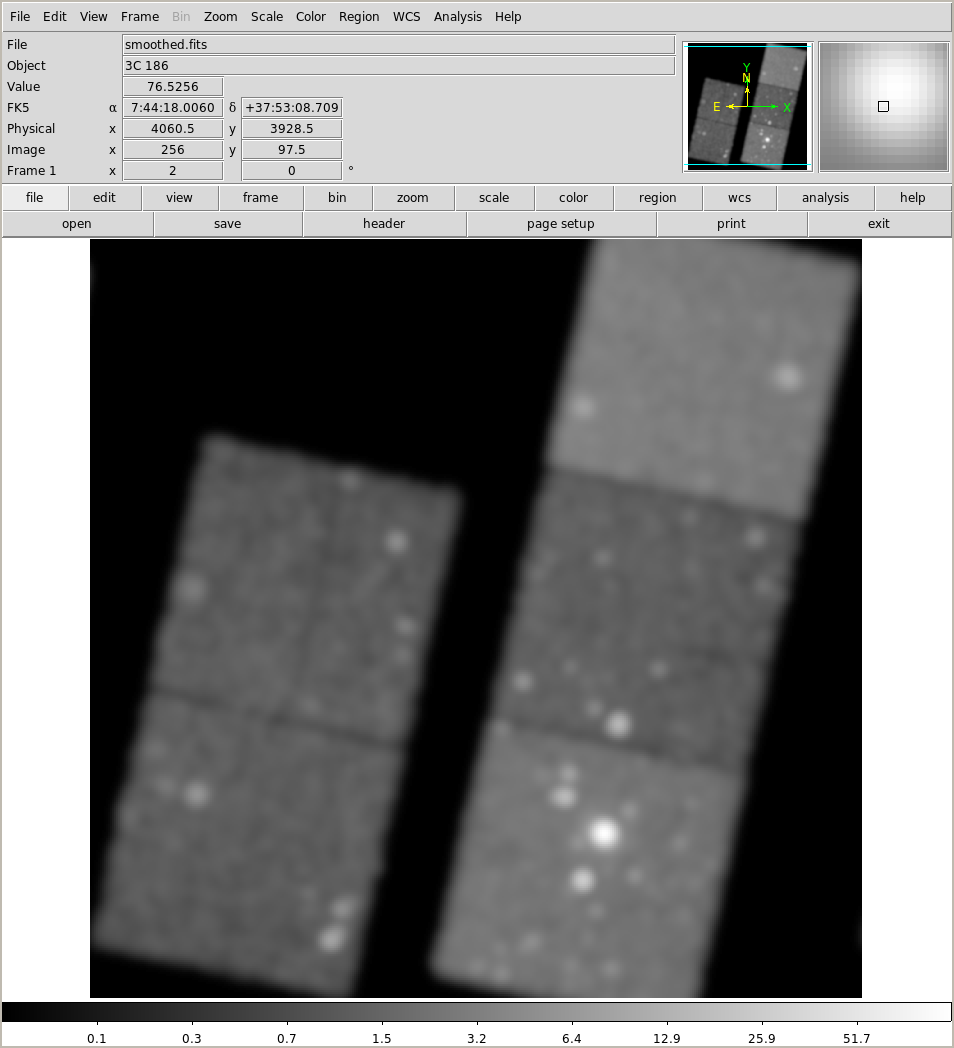
We can try to be clever and use an adaptive-smoothing scheme with the csmooth tool:
https://cxc.cfa.harvard.edu/ciao/ahelp/csmooth.html
(named arguments are used because there are many of them, so it's easier to remember what any one argument is, and also because there's at least one argument I am skipping):
!punlearn csmooth
!csmooth 9774/fluxed/broad_thresh.img outfile=smoothed/adaptive.fits  outsigfile=smoothed/adaptive_sig.fits \
  outsclfile=smoothed/adaptive_scl.fits sigmin=3 mode=h cl+
# WARNING: Kernel cannot be larger than image, setting to size of image
# WARNING: Remainder will be smoothed on scale of 47.986092
This can take noticeably longer than aconcolve, and I am just showing a quick way of running it (please see the ahelp
file and threads for much-more information).
!ds9 smoothed/adaptive_scl.fits -zoom 2 smoothed/adaptive.fits -scale log -cmap viridis
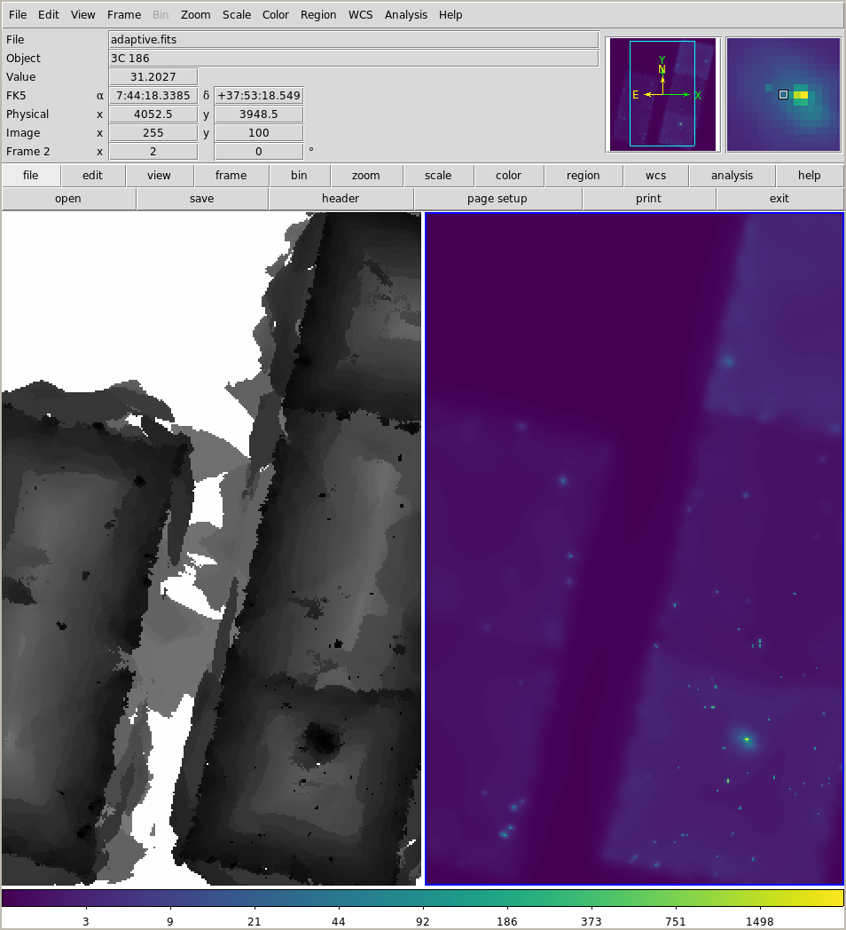
The scale map (left) indicates the scale size used at each location, and you can see it includes areas between the chips.
Interpreting these images is tricky!
There are more ways to bin images (and event files) in CIAO:
https://cxc.harvard.edu/ciao/gallery/binning.html
Radial profile
We need a set of annuli and the dmextract tool:
https://cxc.cfa.harvard.edu/ciao/ahelp/dmextract.html
Note that the CIAO thread Obtain and Fit a Radial Profile should be reviewed and there are a number of Sherpa threads on fitting two-dimensional data (here I am going to focus on one-dimensional data).
!mkdir profile
!punlearn dmextract
!dmextract "9774/fluxed/broad_thresh.img[bin sky=annulus(116.0728015671739d,37.8881248629715d,0:2000:10)]" \
    out=profile/run1.fits opt=generic clob+
The dmextract tool can create spectra, light curves, and radial profiles depending on
- the
optparameter (here it isgeneric) - the
infileargument, in particular thebinargument
The annulus option creates a set of concentric circles, centered on the came position - in this defined
using celestial coordinates as the two values end in a d character - and then covering a range of radii
(in this case 0 to 2000 pixels, with a spacing of 10 pixels). The ACIS pixel size is 0.492 arcseconds on
a side, so 10 pixels represents a width of 4.92 arcseconds.
!dmlist profile/run1.fits blocks
--------------------------------------------------------------------------------
Dataset: profile/run1.fits
--------------------------------------------------------------------------------

     Block Name                          Type         Dimensions
--------------------------------------------------------------------------------
Block    1: PRIMARY                        Null
Block    2: HISTOGRAM                      Table        19 cols x 200      rows
That's a lot of columns!
!dmlist profile/run1.fits cols
--------------------------------------------------------------------------------
Columns for Table Block HISTOGRAM
--------------------------------------------------------------------------------

ColNo  Name                 Unit        Type             Range
   1   sky(X,Y)             pixel        Real8          -Inf:+Inf            Position
   2   EQPOS(RA,Dec)        deg          Real8          -360.0:      360.0   Position
   3   SHAPE                             String[16]                          Region shape type
   4   R[2]                 pixel        Real8(2)       -Inf:+Inf            Radius
   5   RMID                 pixel        Real8          -Inf:+Inf            Mean of valid R[2] values
   6   ROTANG[2]            pixel        Real8(2)       -Inf:+Inf            Angle
   7   COMPONENT                         Int2           -                    Component number
   8   COUNTS               count        Real8          -Inf:+Inf            Counts
   9   ERR_COUNTS           count        Real8          -Inf:+Inf            Error on counts
  10   AREA                 pixel**2     Real8          -Inf:+Inf            Area of extraction
  11   EXPOSURE             s            Real8          -Inf:+Inf            Exposure time of source file
  12   COUNT_RATE           count/s      Real8          -Inf:+Inf            Rate
  13   COUNT_RATE_ERR       count/s      Real8          -Inf:+Inf            Rate Error
  14   NET_COUNTS           count        Real8          -Inf:+Inf            Net Counts
  15   NET_ERR              count        Real8          -Inf:+Inf            Error on Net Counts
  16   NET_RATE             count/s      Real8          -Inf:+Inf            Net Count Rate
  17   ERR_RATE             count/s      Real8          -Inf:+Inf            Error Rate
  18   SUR_BRI              count/pixel**2 Real8          -Inf:+Inf            Net Counts per square pixel
  19   SUR_BRI_ERR          count/pixel**2 Real8          -Inf:+Inf            Error on net counts per square pixel

--------------------------------------------------------------------------------
World Coord Transforms for Columns in Table Block HISTOGRAM
--------------------------------------------------------------------------------

ColNo    Name
4:    CEL_R                = +0 [arcsec] +0.4920 * (R  -0)
5:    CEL_RMID             = +0 [arcsec] +0.4920 * (RMID  -0)
10:   CEL_AREA             = +0 [arcsec**2] +0.2421 * (AREA  -0)
18:   CEL_BRI              = +0 [count/arcsec**2] +4.1311 * (SUR_BRI  -0)
19:   CEL_BRI_ERR          = +0 [count/arcsec**2] +4.1311 * (SUR_BRI_ERR  -0)
Note that a number of columns are transforms of other columns (using the World Coordinate System support in FITS files to allow the radius and area to be displayed in pixels as well as arcseconds).
Let's look at the CEL_RMID and CEL_BRI columns, using Sherpa (it I were
using the Sherpa application we wouldn't need to bother with this line):
from sherpa.astro import ui
This is not a talk on Sherpa (that's next), but the steps we are going to use are
- load data, in this case
x, y, dyvalues - define a model to describe the data
- fit the model to the data
- tweak things by changing the model (e.g. to add features) or adjusting what range of data we fit
ui.load_data('profile/run1.fits[cols cel_rmid,cel_bri,cel_bri_err]')
ui.plot_data(xlog=True, ylog=True)
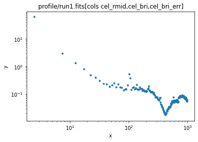
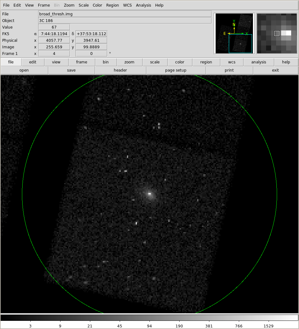
We could try fitting this, but the feature at 400 arcseconds is not easy to model! What is causing this?
!echo 'circle(116.07272d, 37.88809722d, 400")' > profile/circle.reg
!ds9 9774/fluxed/broad_thresh.img -pan to 116.07272 37.88809722 ICRS \
  -zoom 4 -scale log -regions profile/circle.reg
We can see that this dip at ~ 400 arcseconds is related to the gap between the ACIS-S and ACIS-I arrays!
Can we account for this in our modelling or fitting?
There are several ways
- use the exposure map to define those pixels with signal
- filter the event file with the FOV file or the exposure map to store the filter in the subspace of the file: https://cxc.cfa.harvard.edu/ciao/ahelp/subspace.html
Using the exp argument to send in an exposure map to dmextract lets us try the first approach
(note that we use the new CEL_FLUX and CEL_FLUX_ERR columns):
!punlearn dmextract
!dmextract "9774/fluxed/broad_thresh.img[bin sky=annulus(116.0728015671739d,37.8881248629715d,0:2000:10)]" \
    exp=9774/fluxed/broad_thresh.expmap out=profile/run2.fits opt=generic clob+
!dmlist "profile/run2.fits[cols cel_flux,cel_flux_err]" cols
--------------------------------------------------------------------------------
Columns for Table Block HISTOGRAM
--------------------------------------------------------------------------------

ColNo  Name                 Unit        Type             Range
   1   CEL_FLUX             photons/cm**2/arcsec**2/s Real8          -Inf:+Inf
   2   CEL_FLUX_ERR         photons/cm**2/arcsec**2/s Real8          -Inf:+Inf
ui.load_data('profile/run2.fits[cols cel_rmid,cel_flux,cel_flux_err]')
ui.plot_data(xlog=True, ylog=True)
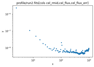
Note that the background is now "more flat" (but not perfectly flat).
Since we are using the flux values the per-bin values are small, so I am going to take a $10^{-9}$ factor outside the models (which helps the fits). First let's get a handle on the background, which I am going to model as a constant:
ui.set_source(1e-9 * ui.const1d.bgnd)
ui.fit()
Dataset               = 1
Method                = levmar
Statistic             = chi2
Initial fit statistic = 96099.5
Final fit statistic   = 11941.2 at function evaluation 4
Data points           = 200
Degrees of freedom    = 199
Probability [Q-value] = 0
Reduced statistic     = 60.0062
Change in statistic   = 84158.3
   bgnd.c0        5.70904      +/- 0.0162324
ui.plot_fit(xlog=True, ylog=True)
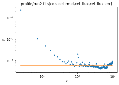
We can now add in a beta1d profile - https://cxc.cfa.harvard.edu/sherpa/ahelp/beta1d.html - which is commonly used to model the X-ray emission of galaxy clusters:
ui.set_source(1e-9 * (bgnd + ui.beta1d.clus))

# help the fit out a bit
clus.r0 = 10
clus.ampl = 100
ui.fit()
Dataset               = 1
Method                = levmar
Statistic             = chi2
Initial fit statistic = 10978.3
Final fit statistic   = 5360.07 at function evaluation 1024
Data points           = 200
Degrees of freedom    = 196
Probability [Q-value] = 0
Reduced statistic     = 27.3473
Change in statistic   = 5618.2
   bgnd.c0        5.65468      +/- 0.0164242
   clus.r0        0.0354291    +/- 0.00114008
   clus.beta      0.573769     +/- 0.00273697
   clus.ampl      6.95986e+07  +/- 0
ui.plot_fit(xlog=True, ylog=True)
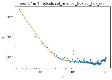
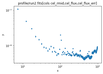
The fit "looks okay", but if you look you can see that the "core radius" (the r0 parameter of the beta1d model) is - to this cluster person - rather small (the axis is in arcseconds so 0.04 arcseconds is a lot smaller than the Chandra PSF). There can be many reasons for this, including the fact that the model may just not be appropriate. I know (from work we've done on this system, and from the image we've seen) that there's a bright QSO at the center of the cluster, and this is likely causing problems, so let's ignore the first bin:
ui.ignore(0, 5)
ui.plot_data(xlog=True, ylog=True)
clus.r0 = 10
clus.ampl = 100

ui.fit()
Dataset               = 1
Method                = levmar
Statistic             = chi2
Initial fit statistic = 5280.15
Final fit statistic   = 5109.11 at function evaluation 58
Data points           = 199
Degrees of freedom    = 195
Probability [Q-value] = 0
Reduced statistic     = 26.2005
Change in statistic   = 171.048
   bgnd.c0        5.59349      +/- 0.0190334
   clus.r0        3.83566      +/- 1.06328
   clus.beta      0.508771     +/- 0.0117872
   clus.ampl      500.723      +/- 212.093
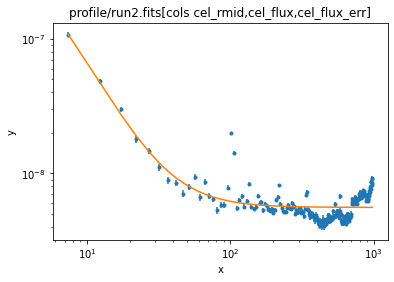
This looks more realistic and still seems to fit the data:
ui.plot_fit(xlog=True, ylog=True)
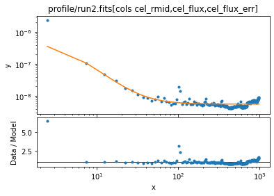
If we add back in the first bin we can see the excess emission that appears to be in the first bin:
ui.notice(None, 5)

ui.plot_fit_ratio(xlog=True, ylog=True)
Things that could be done better
I have not removed point sources from the data, which contributes to the background and some of the spikes.
I am using the default
fluximageoutput, which was binned at 8 ACIS pixels. Since we want to either model, or exclude, the central QSO, we should use a smaller binning factor (if you want to model the PSF then probably so-called "sub-pixel" resolution).The cluster emission is not spherical, so we should use a better model, which could be
use elliptical rather than circluar annuli
fit a two-dimensional model to the date rather than fitting to the profile (e.g. https://cxc.cfa.harvard.edu/sherpa/ahelp/beta2d.html)
Optimize the energy range for the analysis. The data here used the 0.5 - 7.0 keV band range (the so-called
"broad"band), but you may get better results with a lower upper-limit (this depends on the source and background spectra).Use more data.
Better resolution?
Let's quickly look at using smaller pixels (in this case the default 0.492 arcsecond pixel size, and only looking at the "central" chip):
!ls 9774/repro
acisf09774_000N002_bpix1.fits  acisf09774_repro_evt2.fits
acisf09774_000N002_fov1.fits   acisf09774_repro_flt2.fits
acisf09774_000N002_msk1.fits   acisf09774_repro_fov1.fits
acisf09774_000N002_mtl1.fits   acisf313306795N002_pbk0.fits
acisf09774_000N002_stat1.fits  pcadf09774_repro_asol1.fits
acisf09774_asol1.lis	       pcadf313307273N002_asol1.fits
acisf09774_repro_bpix1.fits
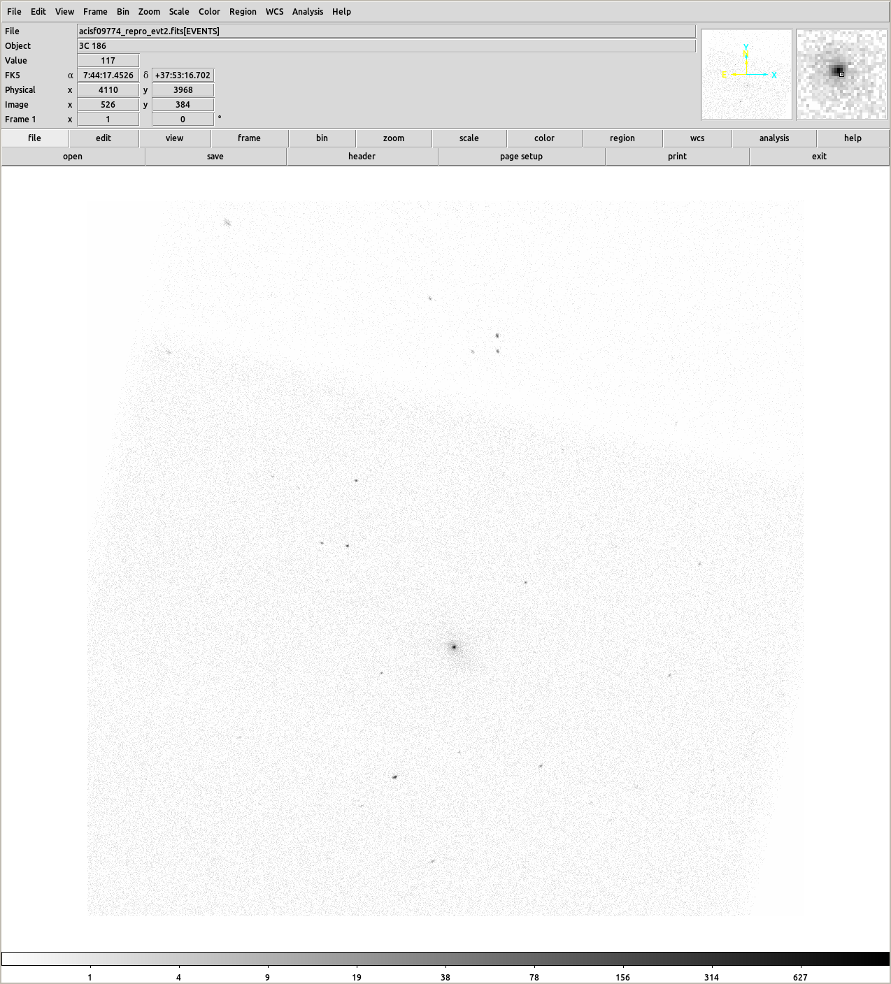
Let's find what chip the cluster is on (spoiler, it's ACIS-S3, also ACIS-7):
!ds9 9774/repro/acisf09774_repro_evt2.fits -scale log
!fluximage "9774/repro/acisf09774_repro_evt2.fits[ccd_id=7]" 9774/ccd7/ bin=1
Running fluximage
Version: 01 April 2020

Using CSC ACIS broad science energy band.
Aspect solution 9774/repro/pcadf09774_repro_asol1.fits found.
Bad-pixel file 9774/repro/acisf09774_repro_bpix1.fits found.
Mask file 9774/repro/acisf09774_000N002_msk1.fits found.

The output images will have 1257 by 1261 pixels, pixel size of 0.492 arcsec,
    and cover x=3422.5:4679.5:1,y=3177.5:4438.5:1.

Running tasks in parallel with 12 processors.
Creating aspect histogram for obsid 9774
Creating instrument map for obsid 9774
Creating exposure map for obsid 9774
Thresholding data for obsid 9774
Exposure-correcting image for obsid 9774

The following files were created:

 The clipped counts image is:
     9774/ccd7/broad_thresh.img

 The clipped exposure map is:
     9774/ccd7/broad_thresh.expmap

 The exposure-corrected image is:
     9774/ccd7/broad_flux.img
For this example I am not going to include an exposure image:
NOTE: the radial bins are narrower, and only extend to r=200 pixel (~100 arcseconds).
!punlearn dmextract
!dmextract "9774/ccd7/broad_thresh.img[bin sky=annulus(116.0728015671739d,37.8881248629715d,0:200:2)]" \
    out=profile/run3.fits opt=generic clob+
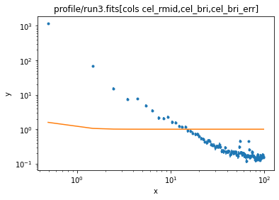
ui.load_data('profile/run3.fits[cols cel_rmid,cel_bri,cel_bri_err]')
ui.set_source(ui.const1d.bgnd2 + ui.beta1d.clus2)
ui.plot_fit(xlog=True, ylog=True)
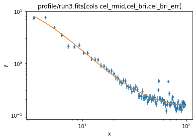
ui.ignore(0, 3)
ui.fit()
Dataset               = 1
Method                = levmar
Statistic             = chi2
Initial fit statistic = 109542
Final fit statistic   = 261.261 at function evaluation 114
Data points           = 97
Degrees of freedom    = 93
Probability [Q-value] = 6.65587e-18
Reduced statistic     = 2.80926
Change in statistic   = 109281
   bgnd2.c0       0.130091     +/- 0.00562411
   clus2.r0       3.22239      +/- 0.56635
   clus2.beta     0.495608     +/- 0.0143645
   clus2.ampl     16.8629      +/- 3.57039
As a reminder, our previous fit reported
bgnd.c0        5.60187      +/- 0.0189266
clus.r0        3.90492      +/- 1.02941
clus.beta      0.5119       +/- 0.0119744
clus.ampl      492.813      +/- 195.968
(and the units of the amplitude are different now).
ui.plot_fit(xlog=True, ylog=True)
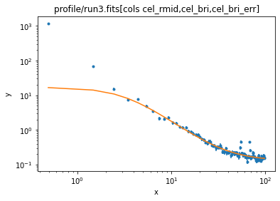
ui.notice()

ui.plot_fit(xlog=True, ylog=True)
If I had time I would talk about including a "point source" model to account for the QSO in the cluster, and fitting a two-dimensional model. There are a number of Sherpa threads that you can read up on!
How can I use more data?
Be VERY careful using dmmerge
https://cxc.cfa.harvard.edu/ciao/ahelp/dmmerge.html
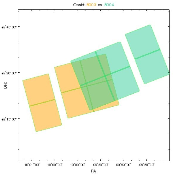
Consider this example of two overlapping (but with separate aim points) ObsIds (we are looking at the outlines of the FOV files):
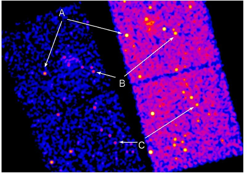
If we just dmmerge the evt2 files we get the following, because the two observations have a different mapping between
SKY coordinates (values ~ 1 - 8192) and celestial coordinates:
We have to reproject the data so that the SKY coordinates make sense:
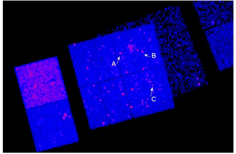
Note that even with reprojection the different datasets are not guaranteed to merge nicely together:
exposure times are normally different
unless the observations have a similar aim point then the PSF size at a given celestial location will differ for the different datasets
background levels can vary when Front-Illuminated and Back-Illuminated chips overlap
Pop Quiz
- Which detector has BI chips?
We used to have a script called merge_all that a user had written that attempted to combine ObsIds, but
it still had issues, and we now strongly recomment that you use merge_obs or the combination of reproject_obs and flux_obs:
https://cxc.cfa.harvard.edu/ciao/ahelp/merge_obs.html
https://cxc.cfa.harvard.edu/ciao/ahelp/reproject_obs.html
https://cxc.cfa.harvard.edu/ciao/ahelp/flux_obs.html
So this should be taken to be a note about all the things that can go wrong when merging data!
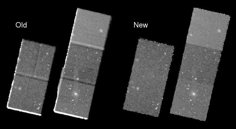
The merge_obs command will
reproject all the ObsIds to an "average" tangent point
create images and exposure maps for each ObsId and each band
combine the images
create a merged event file which SHOULD NOT BE USED TO EXTRACT SPECTRA
If you have multiple CPU cores then it can run relatively fast (especially with its default bin size), but be warned!
Pop Quiz
Why did I list the
FPvalue for each observation (this gives the temperature of the focal-plane instrument for the observation)Does anyone rember Kenny's discussion about SIM_Z values yesterday?
What on earth does
Obsid 3098 has EXPTIME=0.4 and the rest have 3.1mean?
!punlearn merge_obs
!merge_obs "*/repro/" merged/ bands=csc,broad
Running merge_obs
Version: 05 November 2020

Found 3098/repro/acisf03098_repro_evt2.fits
Found 9407/repro/acisf09407_repro_evt2.fits
Found 9408/repro/acisf09408_repro_evt2.fits
Found 9774/repro/acisf09774_repro_evt2.fits
Found 9775/repro/acisf09775_repro_evt2.fits
Verifying 5 observations.
Using CSC ACIS soft science energy band.
Using CSC ACIS medium science energy band.
Using CSC ACIS hard science energy band.
Using CSC ACIS broad science energy band.
Calculating new tangent point.
New tangent point: RA=7h 44m 17.681s Dec=37d 54' 1.26"

Observations to be reprojected:

  Obsid  Obs Date   Exp    DETNAM     SIM_Z    FP   Sepn   PA
                   (ks)                (mm)    (K)   (')  (deg)
---------------------------------------------------------------
1 3098  2002-05-16  34.4 ACIS-7      -190.143 153.3   1.3  -168
2 9407  2007-12-03  66.3 ACIS-23567  -190.140 154.1   0.3   +15
3 9774  2007-12-06  75.1 ACIS-23567  -190.140 154.4   0.3   +12
4 9775  2007-12-08  15.9 ACIS-23567  -190.140 153.6   0.3   +10
5 9408  2007-12-11  39.6 ACIS-23567  -190.143 153.8   0.3   +11

WARNING - EXPTIME values differ:
  Obsid 3098 has EXPTIME=0.4 and the rest have 3.1

Running tasks in parallel with 12 processors.
Reprojecting 5 event files to a common tangent point.
Merging reprojected events files to merged/merged_evt.fits

Calculating the output grid

The merged images will have 394 by 413 pixels, a pixel size of 3.936 arcsec,
    and cover x=2032.5:5184.5:8, y=3208.5:6512.5:8.

Creating the fluxed images for 5 observations in parallel.
Creating aspect histogram for obsid 3098
Creating aspect histograms for obsid 9407
Creating aspect histograms for obsid 9774
Creating aspect histograms for obsid 9775
Creating aspect histograms for obsid 9408
Creating 4 instrument maps for obsid 3098
Creating 20 instrument maps for obsid 9407
Creating 20 instrument maps for obsid 9775
Creating 20 instrument maps for obsid 9774
Creating 20 instrument maps for obsid 9408
Creating 4 exposure maps for obsid 3098
Creating 20 exposure maps for obsid 9407
Creating 20 exposure maps for obsid 9775
Creating 20 exposure maps for obsid 9774
Combining 5 exposure maps for 4 bands (obsid 9407)
Creating 20 exposure maps for obsid 9408
Combining 5 exposure maps for 4 bands (obsid 9775)
Thresholding data for obsid 3098
Combining 5 exposure maps for 4 bands (obsid 9774)
Thresholding data for obsid 9407
Exposure-correcting 4 images for obsid 3098
Thresholding data for obsid 9775
Exposure-correcting 4 images for obsid 9407
Thresholding data for obsid 9774
Exposure-correcting 4 images for obsid 9775
Combining 5 exposure maps for 4 bands (obsid 9408)
Exposure-correcting 4 images for obsid 9774
Thresholding data for obsid 9408
Exposure-correcting 4 images for obsid 9408

Combining 5 observations.

The following files were created:

The co-added clipped counts images are:
     merged/soft_thresh.img
     merged/medium_thresh.img
     merged/hard_thresh.img
     merged/broad_thresh.img

The co-added clipped exposure maps are:
     merged/soft_thresh.expmap
     merged/medium_thresh.expmap
     merged/hard_thresh.expmap
     merged/broad_thresh.expmap

The co-added exposure-corrected images are:
     merged/soft_flux.img
     merged/medium_flux.img
     merged/hard_flux.img
     merged/broad_flux.img

Warning: the merged event file merged/merged_evt.fits
   should not be used to create ARF/RMF/exposure maps because
      the RA_NOM keyword varies by 0.0072 (limit is 0.0003)
      the DEC_NOM keyword varies by 0.0262 (limit is 0.0003)
      the ROLL_NOM keyword varies by 167.9 (limit is 1.0)
      the EXPTIME keyword contains: 0.4 3.1
        which means that the DTCOR value, and hence LIVETIME/EXPOSURE
        keywords are wrong
!ds9 merged/broad_flux.img -scale log -zoom 2 -cmap viridis
This is ~200 ks of data, compared to the 75 ks we have looked at earlier:
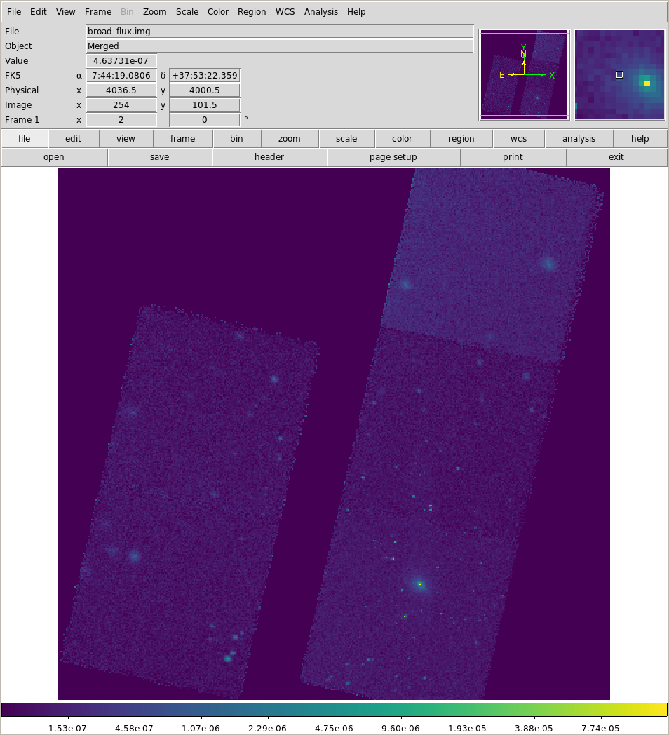
We can also look for spectral differences (Galaxy clusters tend not to show significant broad-band color variations, but the point sources can be more colorful):
!ds9 -scale log -zoom 2 -rgb \
  -red merged/soft_flux.img \
  -green merged/medium_flux.img \
  -blue merged/hard_flux.img
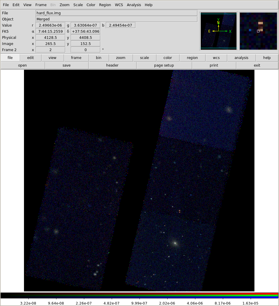
This only scratches the surface. I could
discuss PSF images (e.g. what "is" the PSF size for a point on the sky whem you have overlapping ObsIds)
how do I run source detection on multiple datasets (can we combine, or fit separately)
how do I create spectra for multiple observations?
It is VITALLY IMPORTANT to know when you can use "combined" or "merged" data (such as the images created by merge_obs) and when do we multiple datasets (such as spectral fitting). It depends on how important knowledge of the instrument response for each point on the sky is:
these values can depend on position on the detector (e.g. PSF size or the effective area)
do these values vary with time (e.g. due to the build-up of contamination on the ACIS filter or the detector response as the focal-plane temperature has changed).
Download the notebook.