| PREVIOUS | INDEX | NEXT |
| HETGS Range: | 0.4-10.0 keV, 31-1.2Å |
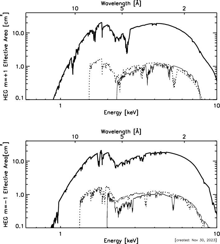
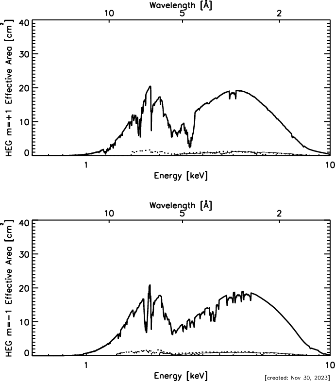
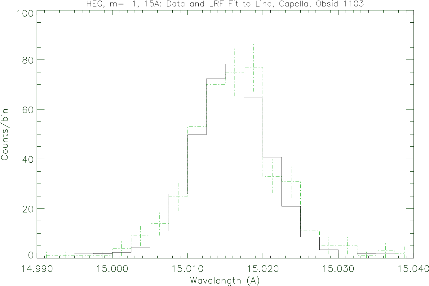
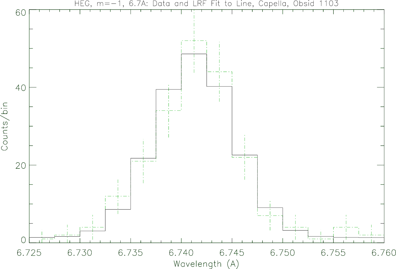
| HEG Range: | 0.8-10.0 keV, 15-1.2 Å |
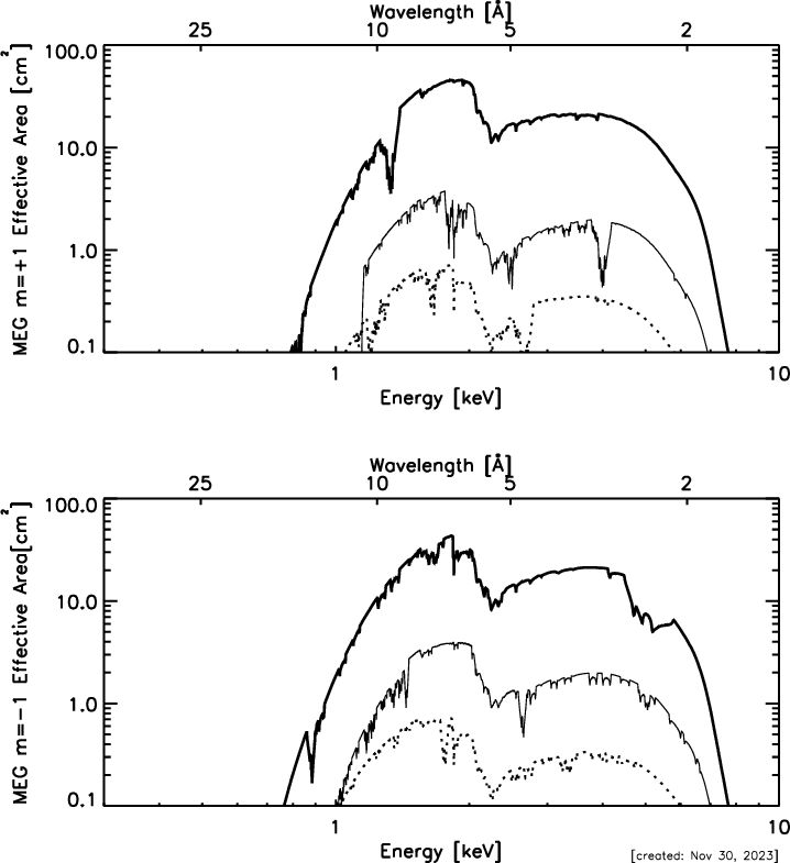
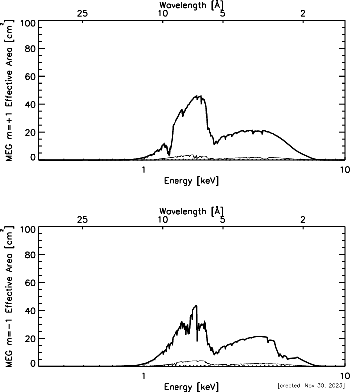
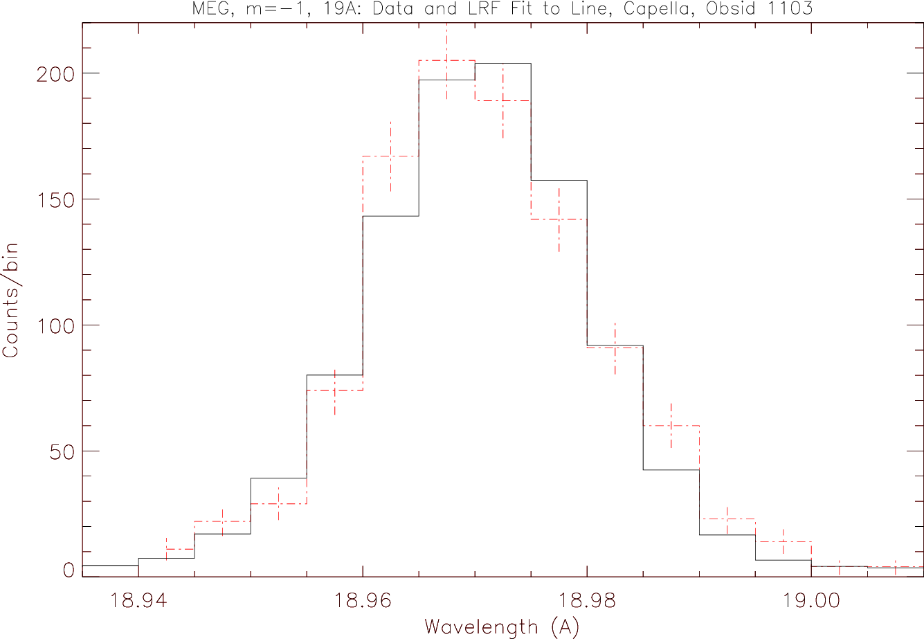
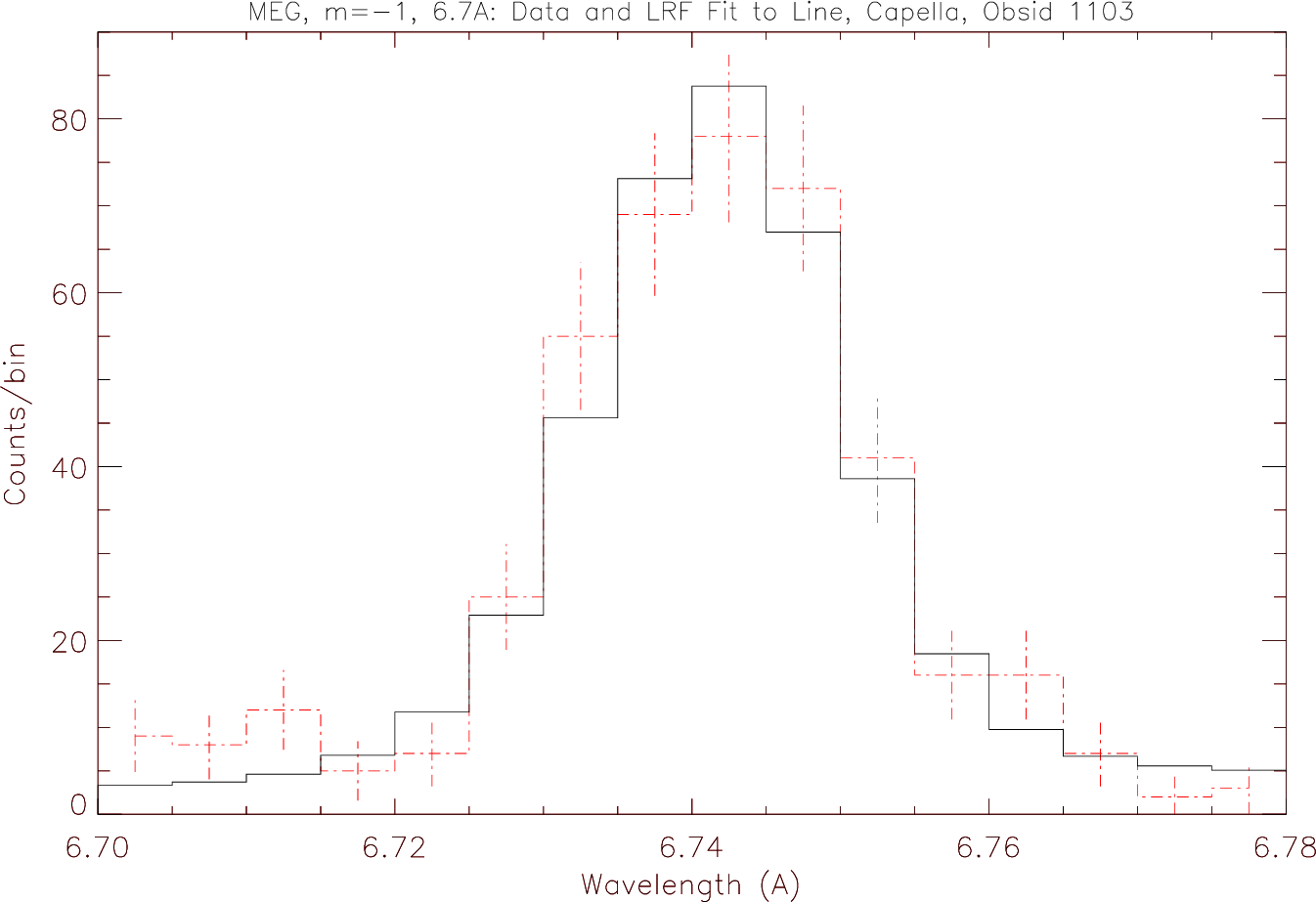
| MEG Range: | 0.4-5.0 keV, 31-2.5 Å |
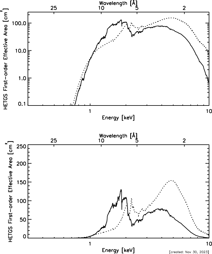
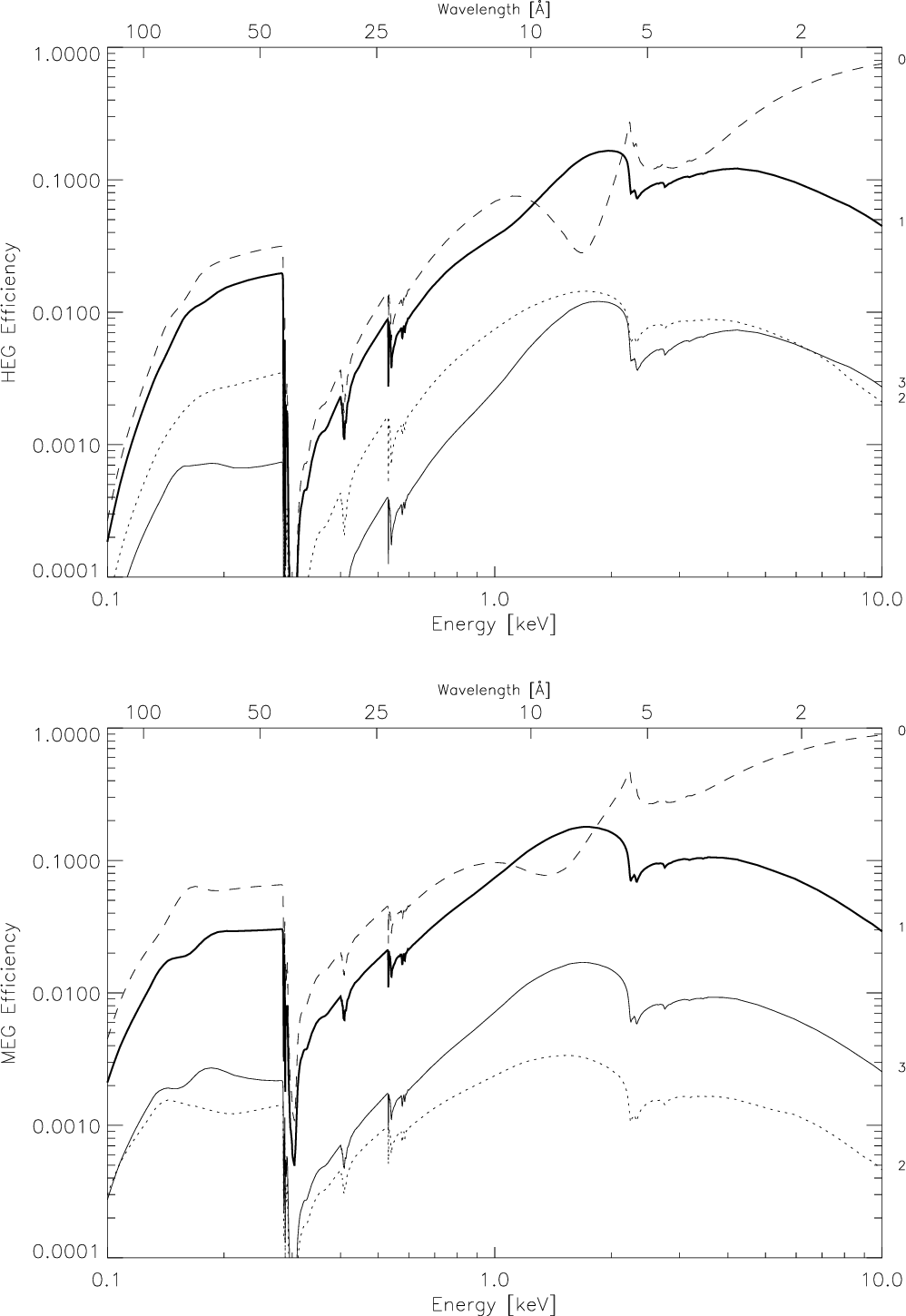
| Effective Area (see Figures 8.7 8.8): | 7 cm2 @ 0.5 keV |
| ( MEG+HEG first orders, | 59 cm2 @ 1.0 keV |
| with ACIS-S) | 200 cm2 @ 1.5 keV |
| 28 cm2 @ 6.5 keV | |
| Resolving Power (E/∆E, λ/∆λ) | |
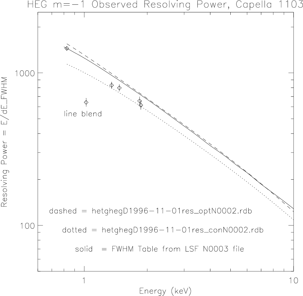
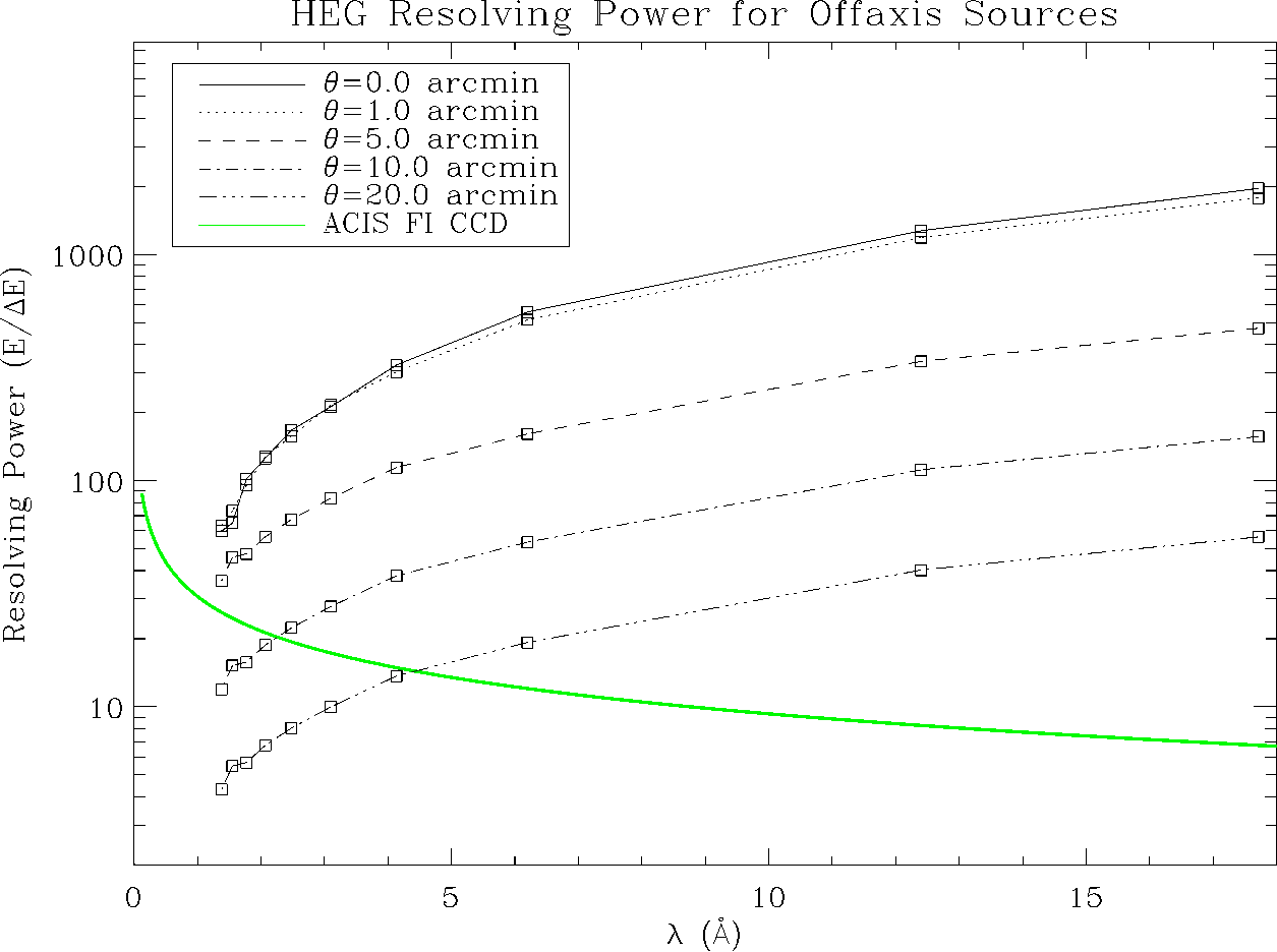
| HEG: | 1070-65 (1000 @ 1 keV, 12.4 Å) |
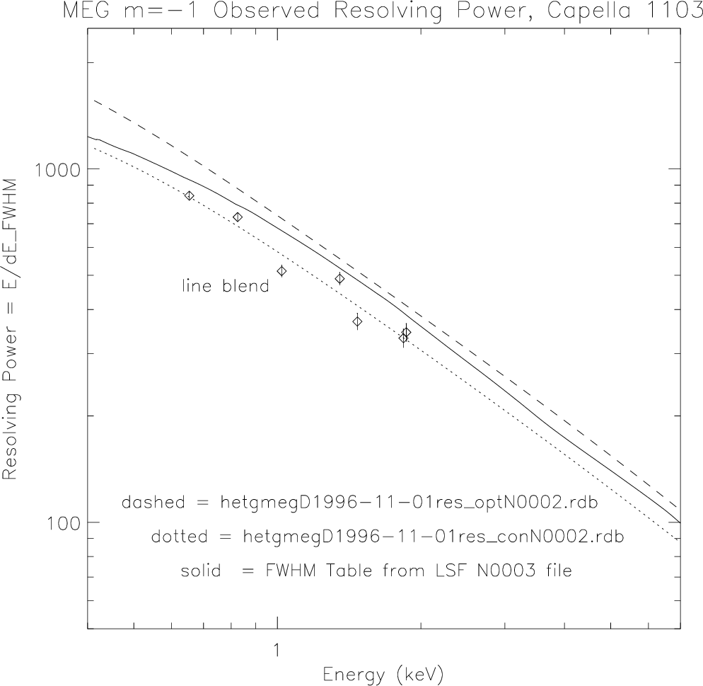
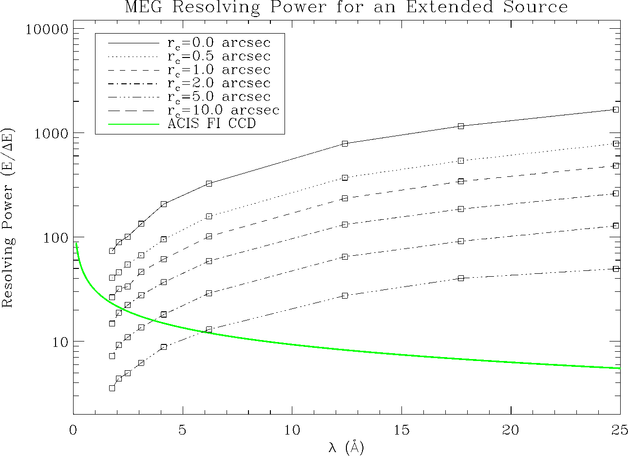
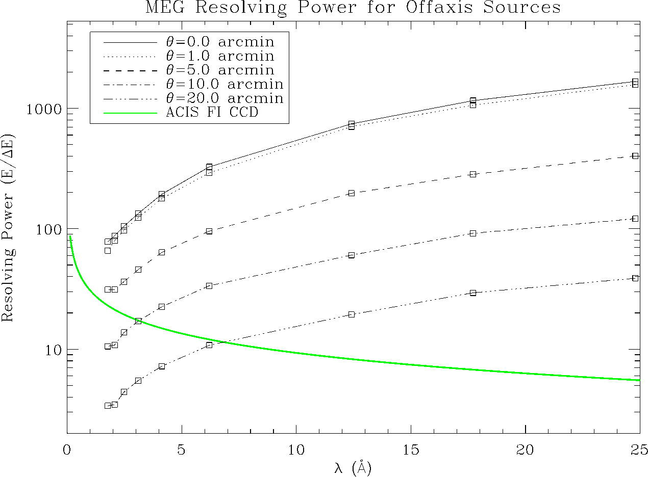
| MEG: | 970-80 (660 @ 0.826 keV, 15 Å) |
| Resolution: | |
| ∆E: | 0.4-77 eV FWHM |
| ∆λ, HEG: | 0.012 Å FWHM |
| ∆λ, MEG: | 0.023 Å FWHM |
| Absolute Wavelength Accuracy: (w.r.t. "theory") | |
| HEG | ±0.006 Å |
| MEG | ±0.011 Å |
| Relative Wavelength Accuracy: (within and between obs.) | |
| HEG | ±0.0010 Å |
| MEG | ±0.0020 Å |
| HEG angle on ACIS-S: | −5.235° ±0.01° |
| MEG angle on ACIS-S: | 4.725° ±0.01° |
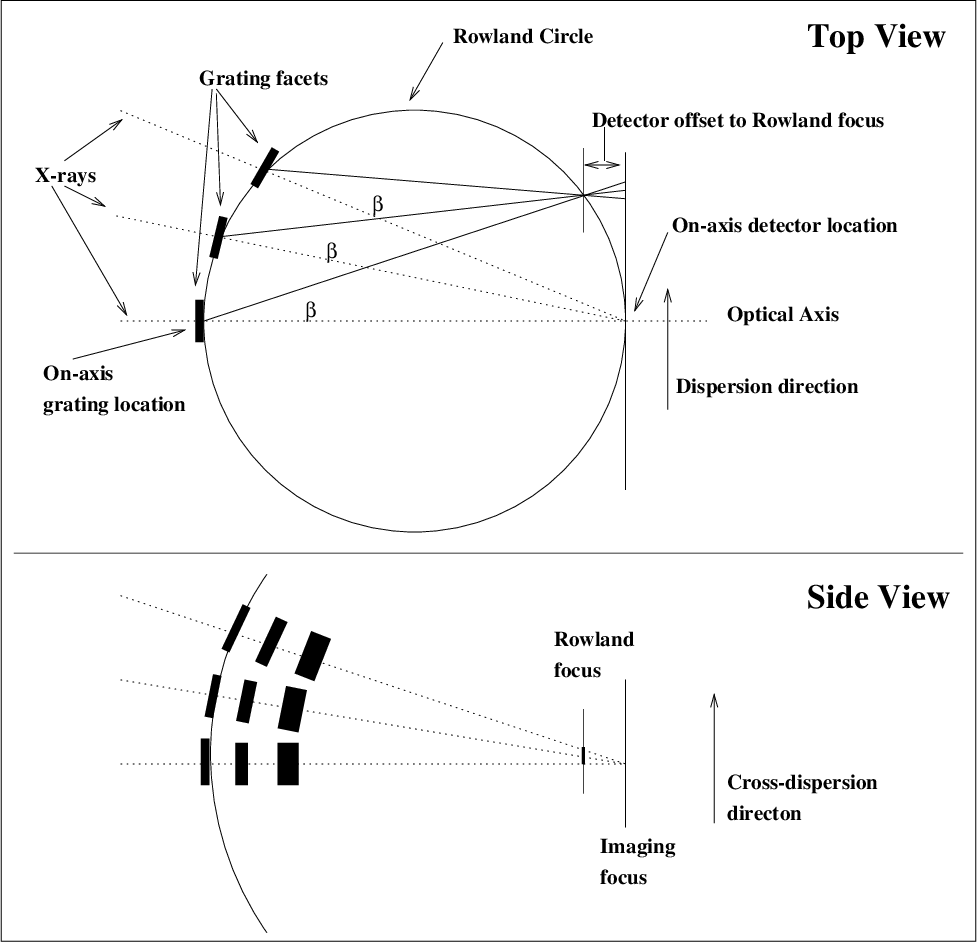
| HETGS Rowland spacing | 8632.65 mm (flight installed) |
| Wavelength Scale: | |
| HEG | 0.0055595 Å / ACIS pixel |
| MEG | 0.0111200 Å / ACIS pixel |
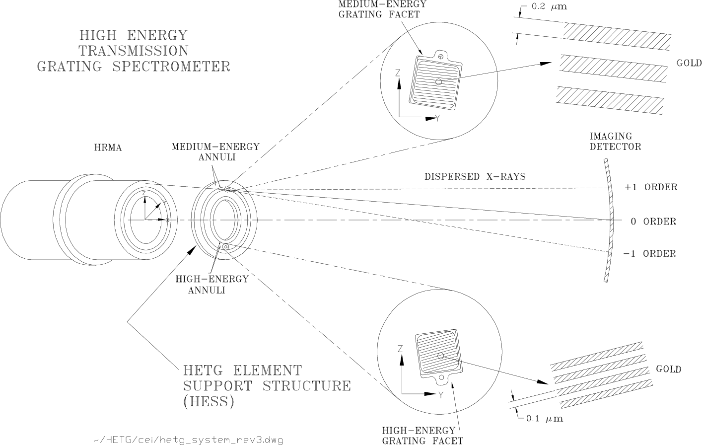
| HETG Properties: | |
| Diffraction Efficiency: | 2.5% @ 0.5 keV (MEG) |
| (single-side, first order) | 19% @ 1.5 keV (MEG & HEG) |
| 9% @ 6.5 keV (HEG) | |
| HETG Zeroth-order Efficiency: | 4.5% @ 0.5 keV |
| 8% @ 1.5 keV | |
| 60% @ 6.5 keV | |
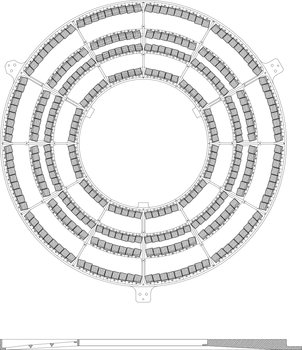
| Grating Facet Average Parameters | |
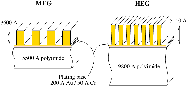
| HEG and MEG bar material: | Gold |
| HEG / MEG period: | 2000.81 Å / 4001.95 Å |
| HEG / MEG Bar thickness: | 5100 Å / 3600 Å |
| HEG / MEG Bar width: | 1200 Å / 2080 Å |
| HEG / MEG support: | 9800 Å / 5500 Å polyimide |
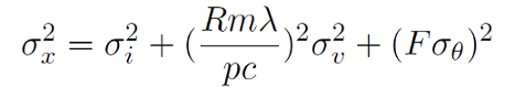
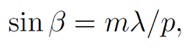 |
(8.1) |
| Y Offset | Grating | HETGS Gaps (keV) | |||||||
| arcmin. | mm | S0 | S0-S1 | S1-S2 | S2-S3 | S3-S4 | S4-S5 | S5 | |
| 1.00 | 2.93 | MEG | 0.508 | 0.969 | 10.724 | 1.183 | 0.561 | 0.367 | |
| 0.346 | 0.512 | 0.987 | 13.439 | 1.157 | 0.555 | ||||
| HEG | 1.014 | 1.937 | 21.434 | 2.364 | 1.120 | 0.734 | |||
| 0.692 | 1.024 | 1.973 | 26.859 | 2.313 | 1.109 | ||||
| 0.66 | 1.93 | MEG | 0.498 | 0.935 | 7.656 | 1.238 | 0.573 | 0.372 | |
| 0.342 | 0.503 | 0.952 | 8.946 | 1.209 | 0.566 | ||||
| HEG | 0.995 | 1.869 | 15.302 | 2.474 | 1.144 | 0.744 | |||
| 0.683 | 1.005 | 1.903 | 17.880 | 2.417 | 1.132 | ||||
| 0.33 | 0.97 | MEG | 0.489 | 0.905 | 5.992 | 1.296 | 0.585 | 0.378 | |
| 0.337 | 0.494 | 0.920 | 6.755 | 1.265 | 0.578 | ||||
| HEG | 0.978 | 1.808 | 11.976 | 2.590 | 1.169 | 0.755 | |||
| 0.674 | 0.987 | 1.839 | 13.500 | 2.528 | 1.156 | ||||
| 0.00 | 0.00 | MEG | 0.481 | 0.876 | 4.923 | 1.360 | 0.597 | 0.383 | |
| 0.333 | 0.485 | 0.891 | 5.426 | 1.326 | 0.591 | ||||
| HEG | 0.961 | 1.751 | 9.838 | 2.718 | 1.194 | 0.765 | |||
| 0.666 | 0.970 | 1.780 | 10.844 | 2.650 | 1.181 | ||||
| −0.33 | −0.97 | MEG | 0.472 | 0.849 | 4.177 | 1.430 | 0.611 | 0.388 | |
| 0.329 | 0.477 | 0.863 | 4.534 | 1.393 | 0.604 | ||||
| HEG | 0.944 | 1.697 | 8.348 | 2.859 | 1.220 | 0.776 | |||
| 0.658 | 0.953 | 1.724 | 9.061 | 2.784 | 1.206 | ||||
| −0.66 | −1.93 | MEG | 0.465 | 0.824 | 3.627 | 1.509 | 0.624 | 0.394 | |
| 0.325 | 0.469 | 0.837 | 3.893 | 1.467 | 0.617 | ||||
| HEG | 0.928 | 1.646 | 7.250 | 3.015 | 1.248 | 0.787 | |||
| 0.650 | 0.937 | 1.672 | 7.781 | 2.932 | 1.233 | ||||
| −1.00 | −2.93 | MEG | 0.457 | 0.799 | 3.194 | 1.599 | 0.639 | 0.400 | |
| 0.322 | 0.461 | 0.811 | 3.399 | 1.552 | 0.632 | ||||
| HEG | 0.913 | 1.597 | 6.384 | 3.195 | 1.278 | 0.799 | |||
| 0.643 | 0.920 | 1.621 | 6.793 | 3.102 | 1.263 | ||||
 |
(8.2) |
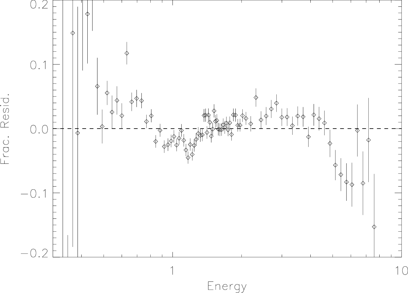
| Energy Range (keV) | r |
| 0.5-1.1 | 0.98 ± 0.05 |
| 1.1-2.4 | 1.02 ± 0.02 |
| 2.4-7.7 | 0.987 ± 0.013 |
 |
(8.3) |
 |
(8.4) |
 |
(8.5) |
| PREVIOUS | INDEX | NEXT |