Gallery: Filter
Examples
- Inline Region Filtering
- Filter using Region File
- Filter Logic: Include and Exclude
- Filter Logic: XOR (Exclusive OR)
- Bounding Box
- Row-|Column-wise projection and replication
- Image Threshold at Zero
- Image Threshold Upper Limit
- Combine Stack of Images: CR rejection
- Background Estimate: Median Ring
- Replace pixels: Interpolation
- Replace Pixels: Random Sample
- Map Based Threshold
1) Inline Region Filtering
Spatial filtering is one of the first operations users typically do. CIAO supports all of the basic region shapes: circle, ellipse, annulus, polygon, box, rectangle, pie, and sector. It supports regions expressed in physical pixels and in World Coordinates. It also supports full Boolean logic between the shapes: union (or), intersection (and), and negation (not).
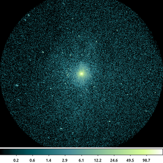
dmcopy "ngc1404.img[sky=circle(3823.5,3959.5,512)]" ngc1404_inline_region.img clob+
The following commands can be used to visualize the output
ds9 ngc1404_inline_region.img -scale log -block 2 -cmap load $ASCDS_CONTRIB/data/green7.lut
In this simple example where we filter on the sky column. The sky column is a virtual, vector column composed of the x and y columns. Since the units of the sky column are in physical pixels, the units of the region are also interpreted as physical pixels.
The region in this example is a single circle that we expressed directly as part of the file name's virtual file syntax.
The default behavior of the CXC datamodel is to set pixel values outside the region to 0, and to reduce the size of the image to the bounding box around the region. Both of these can be changed using the [opt ] directive.
2) Filter using Region File
More complicated regions are often stored in external region files and are read in using the region() syntax.
CIAO supports the ASCII regions that ds9 creates in either the native ds9 format or in the CIAO format. CIAO also supports regions in the ASC-FITS-REGION format.
/bin/rm -f ngc1404_sample.reg
echo "circle(3266,3999,43.326146)" > ngc1404_sample.reg
echo "annulus(3664,4087,49.748272,99.496544)" >> ngc1404_sample.reg
echo "ellipse(3818,3969,69.524371,149.01799,339.1735)" >> ngc1404_sample.reg
echo "box(3425.1778,3885.9166,132.10846,136.39276,27.855707)" >> ngc1404_sample.reg
echo "polygon(3982.0598,3906.9402,4054,4011,4093.9402,3906.9402,4272,3807,4216,3635,3952,3609,3982.0598,3795.0598)" >> ngc1404_sample.reg
echo "pie(3844.4911,4169.4991,0,346.40231,34.028978,87.028978)" >> ngc1404_sample.reg
echo "rectangle(3436.5,3587.5,3598.5,3729.5)" >> ngc1404_sample.reg
dmcopy "ngc1404.img[sky=region(ngc1404_sample.reg)]" ngc1404_regfile.img clob+
The following commands can be used to visualize the output
ds9 ngc1404_regfile.img -region format ciao -region ngc1404_sample.reg -scale log -block 2 -cmap load $ASCDS_CONTRIB/data/green7.lut
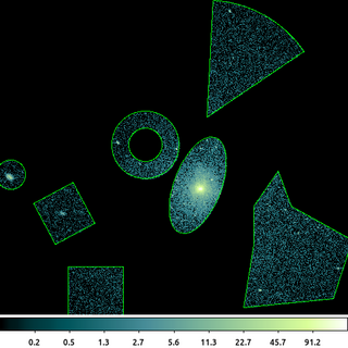
This shows a gallery of most of the CIAO shapes that CIAO supports. The regions are stored in an ASCII file using the simple CIAO format.
The output image shows the input image filtered with the union of the individual shapes. This is the default logic. The individual shapes can also be intersected and/or negated.
The information about the filter is stored in the output file and is used downstream by CIAO in tools such as dmstat and dmextract. You can review the filters by looking at the file's subspace.
dmlist ngc1404_regfile.img subspace
You can get more complicated shapes by inverting regions and by using logical and and or.
3) Filter Logic: Include and Exclude
CIAO regions are composed of individual shapes, eg circles, boxes, ellipses, polygons, etc. These individual shapes can be combined together to create regions using the logic operators AND and OR (or in set-theory terminology Intersections and Unions). Individual shapes can be either included or excluded, ie a logical NOT). In CIAO region syntax the minus operator is equivalent to "AND NOT".
CIAO handles excluded regions differently than some other software packages, including ds9. In CIAO syntax, an excluded shape must be excluded from another, singular, shape whereas in ds9 an excluded shape is excluded from all shapes. It can help to think of CIAO syntax using mathematical operators: AND is multiplication, *, OR is addition, +, and NOT is inversion which we'll indicate as, !. As mentioned, the minus operator is short hand for "AND NOT", or in mathematically terms : *!. Given the usual order of precedence ("*" before "+"), we can then expect that the order that regions are written can make a difference.
This comes up frequently when working with regions created with ds9. The order the regions are written matters.
echo "circle(3683,3950,100)" > trio.reg
echo "-circle(3783,3950,100)" >> trio.reg
echo "circle(3883,3950,100)" >> trio.reg
dmcopy "ngc1404.img[sky=circle(3683,3950,100)-circle(3783,3950,100)+circle(3883,3950,100)]" filter_logic1.img clob+
dmcopy "ngc1404.img[sky=circle(3683,3950,100)+circle(3883,3950,100)-circle(3783,3950,100)]" filter_logic2.img clob+
dmcopy "ngc1404.img[sky=field()-circle(3783,3950,100)+circle(3683,3950,100)+circle(3883,3950,100)]" filter_logic3.img clob+
dmcopy "ngc1404.img[sky=circle(3683,3950,100)-circle(3783,3950,100)+circle(3883,3950,100)-circle(3783,3950,100)]" filter_logic4.img clob+
The following commands can be used to visualize the output
ds9 filter_logic1.img -region trio.reg filter_logic2.img -region trio.reg filter_logic3.img -region trio.reg filter_logic4.img -region trio.reg -tile \
    mode column -frame 1 -scale log -block 2 -cmap load $ASCDS_CONTRIB/data/green7.lut -match colorbar -match block -match scale -view multi no
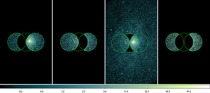
In this example we see the same 3 shapes written in different orders produces different results. For simplicity we'll call the regions: A=circle(3683,3950,100), B=circle(3783,3950,100), and C=circle(3883,3950,100).
Left-most: A-B+C. In this example circle B is excluded from circle A. Writing it out with mathematical operators : A-B+C = A*!B+C = (A*!B)+C.
Left-of-Center: A+C-B. In this example shape B is moved to the end so that it is now only excluded from C: A+C-B = A+C*!B = A+(C*!B).
Right-of-Center: -B+A+C. First thing to note is the addition of the field() shape. Why? Remember that the minus operator is really two: multiplication and negation. So -B+A+C would literally be : *!B+A+C which is nonsensical and is actually illegal syntax. This command
dmcopy "ngc1404.img[sky=-circle(3783,3950,100)+circle(3683,3950,100)+circle(3883,3950,100)]" filter_logic3.img clob+
produces a error: "Bad syntax for region". The field() is added so that the shape has something to be excluded from. Now the expression is: field()-B+A+C = (field()*!B)+A+C. The field() includes everything and the circle is excluded from it; then the pixels inside circle A and circle C are then added back into the filter resulting in the image shown.
Right-most: A-B+C-B. Finally we show how to exclude circle B from both A and C it has to be explicitly expressed that way. A-B+C-B = (A*!B)+(C*!B).
4) Filter Logic: XOR (Exclusive OR)
CIAO regions supports full Boolean logic: and, or, not, operations on individual shapes. This makes CIAO very flexible; but can lead to some confusion for new users.
One of the most common CIAO questions is how excluded regions are treated. In some data analysis systems, an excluded shape is always implicitly excluded from every/any shape it overlaps. This is not how CIAO interprets excluded shapes. Given the full Boolean logic operations available in CIAO, a shape must explicitly be excluded from any/every overlapping shape as required.
This use of explicit logic leads to much greater flexibility in how regions are interpreted. As an example, consider the Exclusive OR operation:
\[ A \oplus B = A\bar{B} + B\bar{A} \]In astronomy terms, this might be used to create a region that includes the flux from two regions, but not the flux from the overlapping region. This operation is difficult to replicate in some systems; however, using the relation shown above, it is simple to perform with CIAO region filters.
/bin/rm -f ngc1404_xor.reg
echo "ellipse(3822.6874,3961.1154,254,52,140)" > ngc1404_xor.reg
echo "-ellipse(3822.6874,3961.1154,254,52,40)" >> ngc1404_xor.reg
echo "ellipse(3822.6874,3961.1154,254,52,40)" >> ngc1404_xor.reg
echo "-ellipse(3822.6874,3961.1154,254,52,140)" >> ngc1404_xor.reg
dmcopy "ngc1404.img[sky=region(ngc1404_xor.reg)][opt full]" ngc1404_xor.img clob+
The following commands can be used to visualize the output
ds9 ngc1404_xor.img -region format ciao -region ngc1404_xor.reg -scale log -block 2 -cmap load $ASCDS_CONTRIB/data/green7.lut
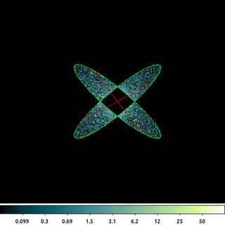
This is the combination of 4 ellipses which have been constructed to create the exclusive OR (XOR) operation. The output retains the data that is in either ellipse, but not both of them. The ellipses are constructed with the same radii and center; the angle (measured from the +X axis) is different.
In CIAO, the minus operator, -, is actually short hand for two separate operations: and and not. So
\[ A-B = A*!B = A*\bar{B} \]Using this we can see how the above filter logic works. The data from the first ellipse is included, except for the region which overlaps the second ellipse. That is then union-ed (OR) with the data from the second ellipse, excluded for the region that overlaps the first ellipse.
This type of logic is not available in some other software systems. By removing the excluded regions, always from every overlapping shape, the result of this region file would be that all pixels would be excluded.
The figure above shows all four ellipses; however, since they overlap only two are visible. Also, since the ellipses are excluded, the red-hash line ds9 uses to indicate negation is seen. ds9 can only display the individual shapes, not the logic used to combine those shapes.
Note the use of [opt full]. The default behavior is to shrink the image to a bounding box around the filtered region, but using the full option the original image size is retained.
5) Bounding Box
There are various use-cases where we only need to know the size and extent of the region being used. These include pre-filtering the dataset to make subsequent filtering faster; getting the size so that other products (exposure maps, PSF maps) can be made on the same grid; determining the set of CCDs being imaged; etc.
The bounds() syntax can be used with any region specifier to get a bounding box around the region. The bounding box is always rectangular and non-rotated. It only considers the region, not the data.
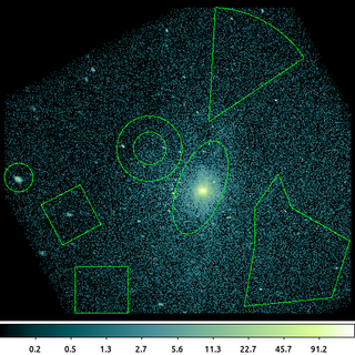
dmcopy "ngc1404.img[sky=bounds(region(ngc1404_sample.reg))]" ngc1404_bounds.img clob+
The following commands can be used to visualize the output
ds9 ngc1404_bounds.img -region format ciao -region ngc1404_sample.reg -scale log -block 2 -zoom 0.95 -cmap load $ASCDS_CONTRIB/data/green7.lut
This is an example of using bounds() using the region file created in the above example. The individual shapes have not been used to construct the filter logic; rather the size/extent of each shape is used to create an overall bounding box around all the shapes in the region file.
The output image has been shrunk to the limits of the bounding box; unlike in the earlier example, the pixels "between" the shapes are included, since the bounds() syntax was used.
6) Row-|Column-wise projection and replication
There are various techniques to determine the background level in an image. ACIS raw images, those used on-orbit for event detection, have strong column-to-column variation and significant offsets between each of the four readout-nodes.
The ACIS on-orbit bias maps are created by taking the average of the pixel values in each column. Only part of the CCD is processed at a time due to the memory limits of the camera.
We can approximate this column-by-column background determination using the dmimgproject and dmimgreproject tools.
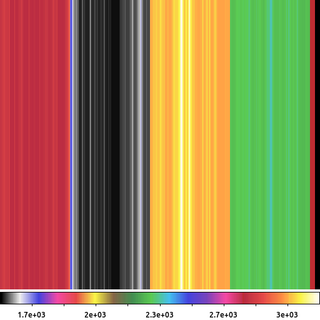
dmimgproject acisf367640304N001_5E002_img0.fits outfile=bias_projx.tab axis=x clob+
dmimgreproject "bias_projx.tab[cols x,mean]" acisf367640304N001_5E002_img0.fits acisf367640304N001_5E002_offset.img method=closest clob+
The following commands can be used to visualize the output
ds9 acisf367640304N001_5E002_offset.img -block 2 -cmap load $ASCDS_CONTRIB/data/pastel.lut
In this example we first take an ACIS raw image, acisf367640304N001_5E002_img0.fits, and compute the projections onto the X-axis. This is an image in ACIS chip coordinates: CHIPX goes along the X-axis and CHIPY along the Y-axis. Data are readout along the CHIPY direction to one of four amplifier nodes. Due to the high dynamic range of pixel values, it is difficult to display this image before background subtraction and therefore not shown here.
Due to the limited telemetry bandwidth, ACIS raw images are rarely telemetered to the ground. Usually, events are detected and the raw image buffer is flushed. However, for calibration and health-and-safety purposes, the CXC collects raw images from ACIS several times per year. Users must request these files from the archive operations group.
dmimgproject computes several statistics for each column (X-axis) or row (Y-axis) including the mean pixel value, median, standard deviation, etc. In this example, to replicate the on-orbit behavior we are going to use the mean value.
In the second command, dmimgreproject is used to replicate the per-column mean value back into each row of the image. The output image shown above. Each column is a constant value equal to the mean of the pixel values in that column. The four ACIS readout nodes are clearly visible as is the column-to-column variation within each node.
The small stripes of data on the far right-hand-side of the image is from the overclock pixels, which are not physically present on the CCD; a full discussion of the topic of overclock pixels is beyond the scope of this example.
7) Image Threshold at Zero
Rather than remove pixels, you may want to replace values in the image. One common approach is to set a threshold and to replace values less than that threshold to some fixed value. For example when subtracting background, you may want to set any residuals <0 to 0.
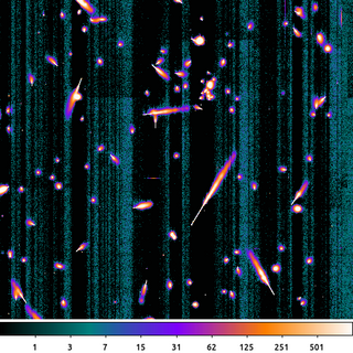
dmimgcalc acisf367640304N001_5E002_img0.fits acisf367640304N001_5E002_offset.img acisf367640304N001_5E002_flat_img0.fits sub clob+
dmimgthresh acisf367640304N001_5E002_flat_img0.fits acisf367640304N001_5E002_zero.img cut=0 value=0 clob+
The following commands can be used to visualize the output
ds9 acisf367640304N001_5E002_zero.img -block 2 -cmap load $ASCDS_CONTRIB/data/icool.lut -scale log -scale limits 0 1000
First, we subtract the output bias map from the previous example from the original raw image. This removes all the node-to-node and column-to-column variations present in the raw exposure.
Then we apply a threshold where any pixels less than 0 are set to 0 using dmimgthresh. This is the image shown here.
What we see here is a ~10 second exposure on one of the front-side illuminated CCDs. The bright features are the result of charge liberated from cosmic rays hitting the CCD. The cosmic rays hit the CCD at various angles which leads to shapes of the charge trail. The point of entry is the narrow end of the charge trail. The charge tail blooms as the cosmic ray travels deeper into the Silicon substrate and further away from the influence of the charge-collecting gate structure.
There are also some low-amplitude, residual, column-by-column features which are acceptable given the other sources of noise in the image.
8) Image Threshold Upper Limit
This example builds on the previous example which applied a threshold to values <0. Now in this example we want to apply an upper threshold.
The bright charge clouds produced by the cosmic rays are transient. They need to be removed if we intend to use this image to compute a mean bias.
There are various ways this can be done. Again, here we simulate what the ACIS camera does on-orbit and simply apply an upper-limit threshold.
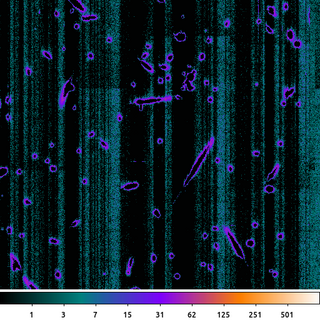
dmimgthresh acisf367640304N001_5E002_zero.img acisf367640304N001_5E002_crater.img cut=:20 value=0 clob+
The following commands can be used to visualize the output
ds9 acisf367640304N001_5E002_crater.img -block 2 -cmap load $ASCDS_CONTRIB/data/icool.lut -scale log -scale limits 0 1000
Here an upper threshold of 20 was applied. But rather than set the pixel values greater than 20 to 20, we instead set them to 0.
This is very similar to the on-board algorithm used to compute the ACIS bias images used for event detection.
The resulting image shown. The idea is that anything greater than this pre-determined threshold must be a cosmic ray. Since we expect the pixel values to be around zero now that we have removed the column-by-column variation, any pixel above a certain threshold is interpreted to be influenced by a cosmic ray charge bloom and the value is replaced with 0.
With the bright, central part of the charge clouds removed; only the edges remain giving the image a cratered look.
9) Combine Stack of Images: CR rejection
If we repeat the previous two steps with several other ACIS raw frames, we can then combine them together to create a final bias map.
The residual column-by-column and cosmic-ray-crater edges can be further suppressed by averaging multiple exposures together.
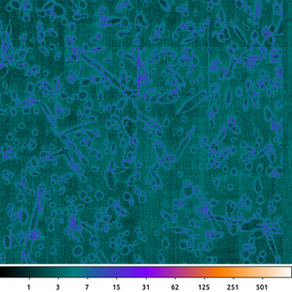
dmimgfilt "acisf367640304N001_5E*crater.img" acisf367640304N001_5_bias.img mean "point(0,0)" clob+
The following commands can be used to visualize the output
ds9 acisf367640304N001_5_bias.img -block 2 -cmap load $ASCDS_CONTRIB/data/icool.lut -scale log -scale limits 0 1000
The previous steps were repeated with the other ACIS raw images. The result is a set of eight images which look similar to this example, each with its own unique pattern of cosmic ray crater edges.
To create the output file, the dmimgfilt tool takes the same point(0,0) from each of the images in the stack, computes the mean of those value and stores it in the output image. It then moves the point to the next pixel and repeats. This stack of input images is specified using the UNIX wildcard, *, syntax: acisf367640304N001_5E*crater.img.
The output then is simply the mean value from the same pixel taken from each file in the input stack. The output is scaled the same as the previous examples so we can see that the amplitude of the residual noise has been greatly decreased. There are still some artifacts.
Here we chose to use the mean to match what is done by the ACIS camera on-orbit. Given the nature of the noise and the limited number of data points, using a median or some type of clipped-mean may provide a flatter bias map.
10) Background Estimate: Median Ring
Non-linear filters can be useful in a variety of ways. The Median Ring technique discussed in the An Estimated Background Image thread is a quick way to get a fairly reliable estimate of image background.
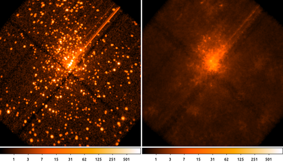
The following commands can be used to visualize the output
ds9 orion.img orion.bkg -frame 1 -scale log -scale limits 0 1000 -block 2 -cmap heat -frame 2 -scale log -scale limits 0 1000 -cmap heat -block 2
This example shows a simple way to estimate the background by computing the median pixel value in an annulus around each pixel in the input image. This process works best when using a smoothed image, since the median of integer values is noisy.
The choice of the size of the annulus (ring) should be such that its inner radius is larger than the expected source size (ie PSF) and the outer radius is small enough to only sample the local background.
We can see in this example that the point sources have been effectively removed from the input image and the diffuse emission at larger spatial scales has been preserved.
This process imparts a low-amplitude, high-spatial frequency structure on the output. If that is undesirable, then users can simply smooth the output
aconvolve orion.bkg orion.sm_bkg "lib:gaus(2,5,5,5,5)"
This type of filter can also be considered a type of non-linear smoothing (taking the median rather than the mean or simple linear combination of values). We can see this in the output as we see the gaps between the chips have increased -- which can be very important when using this type of image for exposure corrections.
11) Replace pixels: Interpolation
Another way to replace the pixel values is to interpolate over some region.
The dmfilth, Fill in the Hole, tool has several options to replace pixels values in the image based on a user supplied background region. Different methods place different restrictions on how the target (ie source) and donor (ie background) regions have to be created.
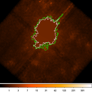
dmimglasso orion.bkg orion.de x=4130 y=4170 lo=0.5 high=INDEF maxdep=100000000 clob+ mode=h
dmimglasso orion.bkg orion.outer_de x=4130 y=4170 lo=0.4 high=INDEF maxdep=100000000 clob+ mode=h
dmcopy orion.outer_de"[region][#row=1]" orion.outer_de.fits clob+
dmcopy orion.de"[region][#row=1]" orion.de.fits clob+
dmfilth orion.bkg orion_interp.bkg method=POLY src="region(orion.de.fits)" bkg="region(orion.outer_de.fits)" mode=h clob+
The following commands can be used to visualize the output
ds9 orion_interp.bkg -scale log -scale limits 0 1000 -cmap heat -block 2 -region orion.outer_de.fits -region color white -region orion.de.fits
In this example we start by running dmimglasso to get a polygon region surrounding the diffuse emission in the background from the previous example. We actually run dmimglasso twice. Once to get an inner polygon, using a higher threshold of 0.5. This is the inner polygon; the pixel values inside this region will be filled in. Then we run dmimglasso again with a lower threshold of 0.4 to generate the outer polygon. The pixel values inside this region (but outside the interior polygon) will be used to compute the coefficients for the two-dimension second-order polygon.
Next we select only the first row of each of those region files using dmcopy. As we saw in another example the dmimglasso output may contain interior excluded regions. For this example we only want the outermost region which will be the first one in the output file.
Finally we then run dmfilth to fill in the hole. Using method=POLY it takes the pixel values in the background region (green polygon) that are not in the source region (white polygon) and uses them to do a 2D, second-order polygonal least-squares-fit over the source region.
12) Replace Pixels: Random Sample
dmfilth also has the option to fill in the source region with random Poisson noise (background).
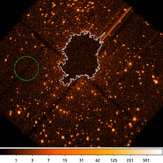
dmfilth "acisf04396_broad_thresh.img[bin sky=2]" orion.poisson_filled.fits method=POISSON src="region(orion.de.fits)" bkg="circle(3435.5,4093.5,150)" rand=32 mode=h clob+
The following commands can be used to visualize the output
ds9 orion.poisson_filled.fits -scale log -scale limits 0 1000 -cmap heat -block 2 -region color white -region orion.de.fits -regions command \
    "circle(3435.5,4093.5,150) # background"
In this example we take the regions from the previous example for the diffuse emission region (white curve) and replace the pixel values by sampling from a Poisson random variable using a count-rate determined from the events in the background (dashed green) region.
dmfilth requires that the background region must be completely disjoint from the source region when using method=POISSON. A co-located annulus is OK as long as there are no pixels at the edge which are included in both regions.
13) Map Based Threshold
The dmimglasso output file contains both a REGION extension as well as a pixel mask that identifies which pixels are inside the region. We can use this to help visualize the polygon region shown in the above example.
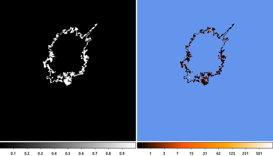
dmimgcalc orion.outer_de orion.de orion.poly_ring sub clob+
dmimgthresh orion.img orion.poly_ring.img cut=1 value=INDEF exp=orion.poly_ring clob+
The following commands can be used to visualize the output
ds9 orion.poly_ring orion.poly_ring.img -frame 1 -zoom 0.5 -frame 2 -nan cornflowerblue -scale log -scale limits 0 1000 -cmap heat -zoom 0.5
(Left) First we subtract the inner polygon from the outer polygon. Since they both started at the same location, the inner polygon must be entirely enclosed within the other polygon. Since the mask pixel values are either 1 (inside the polygon) or 0 (outside), if we subtract the inner mask from the outer mask, the polygon annulus that is left behind will be the region that is inside the outer polygon, but not inside the inner polygon.
(Right) Next we use the subtracted mask to filter the image using dmimgthresh. We set the expfile parameter to the mask file name. Then we set the threshold so that any pixels less than 1 are set to INDEF, which is the special value we use when we want the output pixel values to be NaN or BLANK (depending on the data-type).
The final image shows the filtered data using the ds9 heat color map. Pixel values that are outside the filtered region have been set to NaN and are colored blue.